

934
Appendix: All Solutions to the Problems
δ J =
V
∂ F
∂u
− ∇ · (∇v × c)
δu +
∂ F
∂v
− ∇ · (c × ∇u)
δv
+∇ · [(∇v × c)δu] + ∇ · [(c × ∇u)δv]}dV
(4)
The Euler equations of the functional are
⎧
⎨
⎩
∂ F
∂u
− ∇ ·
∇v ×
∂ F
∂(∇u×∇v)
= 0
∂ F
∂v
+ ∇ ·
∇u ×
∂ F
∂(∇u×∇v)
= 0
(5)
The natural boundary conditions are
∇v ×
∂ F
∂(∇u × ∇v)
· n
S
= 0,
∇u ×
∂ F
∂(∇u × ∇v)
· n
S
= 0
(6)
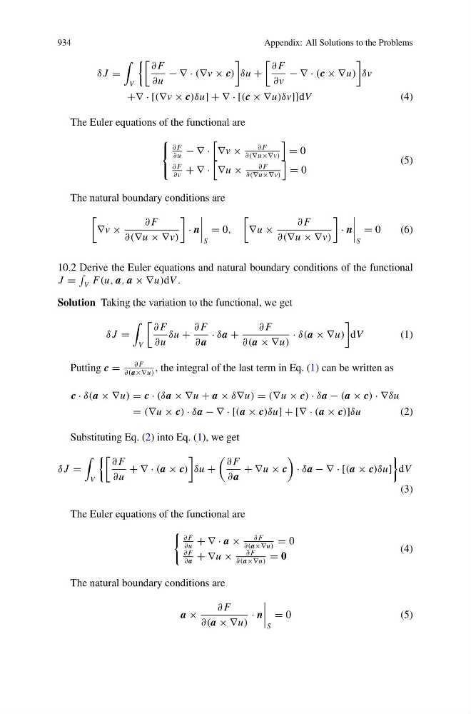
10.2 Derive the Euler equations and natural boundary conditions of the functional
J =
V F(u, a, a × ∇u)dV .
Solution Taking the variation to the functional, we get
δ J =
V
∂ F
∂u
δu +
∂ F
∂ a
· δa +
∂ F
∂(a × ∇u)
· δ(a × ∇u)
dV
(1)
Putting c =
∂ F
∂(a×∇u)
, the integral of the last term in Eq. (1) can be written as
c · δ(a × ∇u) = c · (δa × ∇u + a × δ∇u) = (∇u × c) · δa − (a × c) · ∇δu
= (∇u × c) · δa − ∇ · [(a × c)δu] + [∇ · (a × c)]δu
(2)
Substituting Eq. (2) into Eq. (1), we get
δ J =
V
∂ F
∂u
+ ∇ · (a × c)
δu +
∂ F
∂ a
+ ∇u × c
· δa − ∇ · [(a × c)δu]
dV
(3)
The Euler equations of the functional are
∂ F
∂u
+ ∇ · a ×
∂ F
∂(a×∇u)
= 0
∂ F
∂ a
+ ∇u ×
∂ F
∂(a×∇u)
= 0
(4)
The natural boundary conditions are
a ×
∂ F
∂(a × ∇u)
· n
S
= 0
( 5 )
Appendix: All Solutions to the Problems
δ J =
V
∂ F
∂u
− ∇ · (∇v × c)
δu +
∂ F
∂v
− ∇ · (c × ∇u)
δv
+∇ · [(∇v × c)δu] + ∇ · [(c × ∇u)δv]}dV
(4)
The Euler equations of the functional are
⎧
⎨
⎩
∂ F
∂u
− ∇ ·
∇v ×
∂ F
∂(∇u×∇v)
= 0
∂ F
∂v
+ ∇ ·
∇u ×
∂ F
∂(∇u×∇v)
= 0
(5)
The natural boundary conditions are
∇v ×
∂ F
∂(∇u × ∇v)
· n
S
= 0,
∇u ×
∂ F
∂(∇u × ∇v)
· n
S
= 0
(6)
10.2 Derive the Euler equations and natural boundary conditions of the functional
J =
V F(u, a, a × ∇u)dV .
Solution Taking the variation to the functional, we get
δ J =
V
∂ F
∂u
δu +
∂ F
∂ a
· δa +
∂ F
∂(a × ∇u)
· δ(a × ∇u)
dV
(1)
Putting c =
∂ F
∂(a×∇u)
, the integral of the last term in Eq. (1) can be written as
c · δ(a × ∇u) = c · (δa × ∇u + a × δ∇u) = (∇u × c) · δa − (a × c) · ∇δu
= (∇u × c) · δa − ∇ · [(a × c)δu] + [∇ · (a × c)]δu
(2)
Substituting Eq. (2) into Eq. (1), we get
δ J =
V
∂ F
∂u
+ ∇ · (a × c)
δu +
∂ F
∂ a
+ ∇u × c
· δa − ∇ · [(a × c)δu]
dV
(3)
The Euler equations of the functional are
∂ F
∂u
+ ∇ · a ×
∂ F
∂(a×∇u)
= 0
∂ F
∂ a
+ ∇u ×
∂ F
∂(a×∇u)
= 0
(4)
The natural boundary conditions are
a ×
∂ F
∂(a × ∇u)
· n
S
= 0
( 5 )