

900
Appendix: All Solutions to the Problems
Equation (8) is the same as the exact solution of elastic mechanics.
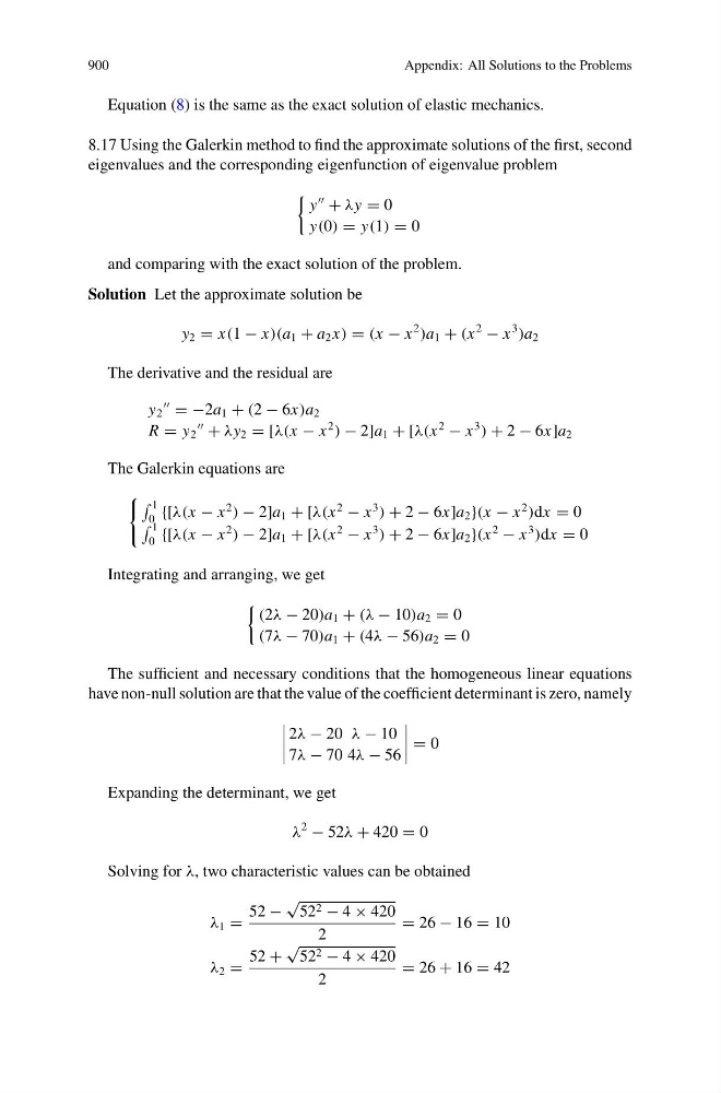
8.17 Using the Galerkin method to find the approximate solutions of the first, second
eigenvalues and the corresponding eigenfunction of eigenvalue problem
y
+ λy = 0
y(0) = y(1) = 0
and comparing with the exact solution of the problem.
Solution Let the approximate solution be
y 2 = x(1 − x)(a 1 + a 2 x) = (x − x
2
)a 1 + (x
2
− x
3
)a 2
The derivative and the residual are
y 2
= −2a 1 + (2 − 6x)a 2
R = y 2
+ λy 2 = [λ(x − x
2
) − 2]a 1 + [λ(x
2
− x
3
) + 2 − 6x]a 2
The Galerkin equations are
1
0 {[λ(x − x
2
) − 2]a 1 + [λ(x
2
− x
3
) + 2 − 6x]a 2 }(x − x
2
)dx = 0
1
0 {[λ(x − x
2
) − 2]a 1 + [λ(x
2
− x
3
) + 2 − 6x]a 2 }(x
2
− x
3
)dx = 0
Integrating and arranging, we get
(2λ − 20)a 1 + (λ − 10)a 2 = 0
(7λ − 70)a 1 + (4λ − 56)a 2 = 0
The sufficient and necessary conditions that the homogeneous linear equations
have non-null solution are that the value of the coefficient determinant is zero, namely
2λ − 20 λ − 10
7λ − 70 4λ − 56
= 0
Expanding the determinant, we get
λ
2
− 52λ + 420 = 0
Solving for λ, two characteristic values can be obtained
λ 1 =
52 −
√
52 2 − 4 × 420
2
= 26 − 16 = 10
λ 2 =
52 +
√
52 2 − 4 × 420
2
= 26 + 16 = 42
Appendix: All Solutions to the Problems
Equation (8) is the same as the exact solution of elastic mechanics.
8.17 Using the Galerkin method to find the approximate solutions of the first, second
eigenvalues and the corresponding eigenfunction of eigenvalue problem
y
+ λy = 0
y(0) = y(1) = 0
and comparing with the exact solution of the problem.
Solution Let the approximate solution be
y 2 = x(1 − x)(a 1 + a 2 x) = (x − x
2
)a 1 + (x
2
− x
3
)a 2
The derivative and the residual are
y 2
= −2a 1 + (2 − 6x)a 2
R = y 2
+ λy 2 = [λ(x − x
2
) − 2]a 1 + [λ(x
2
− x
3
) + 2 − 6x]a 2
The Galerkin equations are
1
0 {[λ(x − x
2
) − 2]a 1 + [λ(x
2
− x
3
) + 2 − 6x]a 2 }(x − x
2
)dx = 0
1
0 {[λ(x − x
2
) − 2]a 1 + [λ(x
2
− x
3
) + 2 − 6x]a 2 }(x
2
− x
3
)dx = 0
Integrating and arranging, we get
(2λ − 20)a 1 + (λ − 10)a 2 = 0
(7λ − 70)a 1 + (4λ − 56)a 2 = 0
The sufficient and necessary conditions that the homogeneous linear equations
have non-null solution are that the value of the coefficient determinant is zero, namely
2λ − 20 λ − 10
7λ − 70 4λ − 56
= 0
Expanding the determinant, we get
λ
2
− 52λ + 420 = 0
Solving for λ, two characteristic values can be obtained
λ 1 =
52 −
√
52 2 − 4 × 420
2
= 26 − 16 = 10
λ 2 =
52 +
√
52 2 − 4 × 420
2
= 26 + 16 = 42