

886
Appendix: All Solutions to the Problems
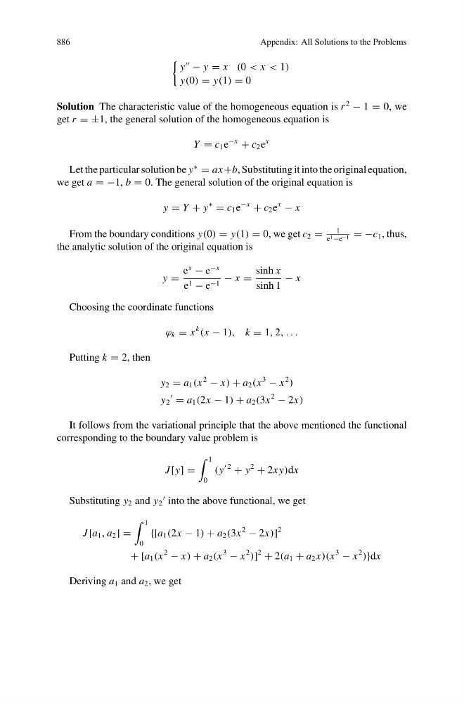
y
− y = x (0 < x < 1)
y(0) = y(1) = 0
Solution The characteristic value of the homogeneous equation is r
2
− 1 = 0, we
get r = ±1, the general solution of the homogeneous equation is
Y = c 1 e
−x
+ c 2 e
x
Let the particular solution be y
∗
= ax+b, Substituting it into the original equation,
we get a = −1, b = 0. The general solution of the original equation is
y = Y + y
∗
= c 1 e
−x
+ c 2 e
x
− x
From the boundary conditions y(0) = y(1) = 0, we get c 2 =
1
e 1 −e −1 = −c 1 , thus,
the analytic solution of the original equation is
y =
e
x
− e
−x
e 1 − e −1 − x =
sinh x
sinh 1
− x
Choosing the coordinate functions
ϕ k = x
k
(x − 1), k = 1, 2, . . .
Putting k = 2, then
y 2 = a 1 (x
2
− x) + a 2 (x
3
− x
2
)
y 2
= a 1 (2x − 1) + a 2 (3x
2
− 2x)
It follows from the variational principle that the above mentioned the functional
corresponding to the boundary value problem is
J [y] =
1
0
(y
2
+ y
2
+ 2x y)dx
Substituting y 2 and y 2
into the above functional, we get
J [a 1 , a 2 ] =
1
0
{[a 1 (2x − 1) + a 2 (3x
2
− 2x)]
2
+ [a 1 (x
2
− x) + a 2 (x
3
− x
2
)]
2
+ 2(a 1 + a 2 x)(x
3
− x
2
)}dx
Deriving a 1 and a 2 , we get
Appendix: All Solutions to the Problems
y
− y = x (0 < x < 1)
y(0) = y(1) = 0
Solution The characteristic value of the homogeneous equation is r
2
− 1 = 0, we
get r = ±1, the general solution of the homogeneous equation is
Y = c 1 e
−x
+ c 2 e
x
Let the particular solution be y
∗
= ax+b, Substituting it into the original equation,
we get a = −1, b = 0. The general solution of the original equation is
y = Y + y
∗
= c 1 e
−x
+ c 2 e
x
− x
From the boundary conditions y(0) = y(1) = 0, we get c 2 =
1
e 1 −e −1 = −c 1 , thus,
the analytic solution of the original equation is
y =
e
x
− e
−x
e 1 − e −1 − x =
sinh x
sinh 1
− x
Choosing the coordinate functions
ϕ k = x
k
(x − 1), k = 1, 2, . . .
Putting k = 2, then
y 2 = a 1 (x
2
− x) + a 2 (x
3
− x
2
)
y 2
= a 1 (2x − 1) + a 2 (3x
2
− 2x)
It follows from the variational principle that the above mentioned the functional
corresponding to the boundary value problem is
J [y] =
1
0
(y
2
+ y
2
+ 2x y)dx
Substituting y 2 and y 2
into the above functional, we get
J [a 1 , a 2 ] =
1
0
{[a 1 (2x − 1) + a 2 (3x
2
− 2x)]
2
+ [a 1 (x
2
− x) + a 2 (x
3
− x
2
)]
2
+ 2(a 1 + a 2 x)(x
3
− x
2
)}dx
Deriving a 1 and a 2 , we get