

Appendix: All Solutions to the Problems
861
namely F(x, y, ˙
x, ˙
y) is the positively homogeneous function of order one about ˙
x
and ˙
y, of course it is also the positively homogeneous function of order one about x
and y, thus The area A of the plane figure surrounded by the closed curve Γ is only
related to the shape of the curve, but it has nothing to do with the parameter form of
the curve Γ . Quod erat demonstrandum.
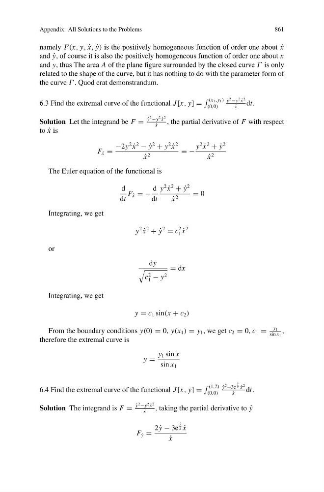
6.3 Find the extremal curve of the functional J [x, y] =
(x 1 ,y 1 )
(0,0)
˙
y
2 −y
2 ˙
x
2
˙
x
dt.
Solution Let the integrand be F =
˙
y
2 −y
2 ˙
x
2
˙
x
, the partial derivative of F with respect
to ˙
x is
F ˙
x =
−2y
2
˙
x
2
− ˙
y
2
+ y
2
˙
x
2
˙
x 2
= −
y
2
˙
x
2
+ ˙
y
2
˙
x 2
The Euler equation of the functional is
d
dt
F ˙
x = −
d
dt
y
2
˙
x
2
+ ˙
y
2
˙
x 2
= 0
Integrating, we get
y
2
˙
x
2
+ ˙
y
2
= c
2
1 ˙
x
2
or
dy
c
2
1 − y 2
= dx
Integrating, we get
y = c 1 sin(x + c 2 )
From the boundary conditions y(0) = 0, y(x 1 ) = y 1 , we get c 2 = 0, c 1 =
y 1
sin x 1
,
therefore the extremal curve is
y =
y 1 sin x
sin x 1
6.4 Find the extremal curve of the functional J [x, y] =
(1,2)
(0,0)
˙
y
2 −3e
˙
y
˙
x ˙
x
2
˙
x
dt.
Solution The integrand is F =
˙
y
2 −y
2 ˙
x
2
˙
x
, taking the partial derivative to ˙
y
F ˙
y =
2 ˙
y − 3e
˙
y
˙
x ˙
x
˙
x
861
namely F(x, y, ˙
x, ˙
y) is the positively homogeneous function of order one about ˙
x
and ˙
y, of course it is also the positively homogeneous function of order one about x
and y, thus The area A of the plane figure surrounded by the closed curve Γ is only
related to the shape of the curve, but it has nothing to do with the parameter form of
the curve Γ . Quod erat demonstrandum.
6.3 Find the extremal curve of the functional J [x, y] =
(x 1 ,y 1 )
(0,0)
˙
y
2 −y
2 ˙
x
2
˙
x
dt.
Solution Let the integrand be F =
˙
y
2 −y
2 ˙
x
2
˙
x
, the partial derivative of F with respect
to ˙
x is
F ˙
x =
−2y
2
˙
x
2
− ˙
y
2
+ y
2
˙
x
2
˙
x 2
= −
y
2
˙
x
2
+ ˙
y
2
˙
x 2
The Euler equation of the functional is
d
dt
F ˙
x = −
d
dt
y
2
˙
x
2
+ ˙
y
2
˙
x 2
= 0
Integrating, we get
y
2
˙
x
2
+ ˙
y
2
= c
2
1 ˙
x
2
or
dy
c
2
1 − y 2
= dx
Integrating, we get
y = c 1 sin(x + c 2 )
From the boundary conditions y(0) = 0, y(x 1 ) = y 1 , we get c 2 = 0, c 1 =
y 1
sin x 1
,
therefore the extremal curve is
y =
y 1 sin x
sin x 1
6.4 Find the extremal curve of the functional J [x, y] =
(1,2)
(0,0)
˙
y
2 −3e
˙
y
˙
x ˙
x
2
˙
x
dt.
Solution The integrand is F =
˙
y
2 −y
2 ˙
x
2
˙
x
, taking the partial derivative to ˙
y
F ˙
y =
2 ˙
y − 3e
˙
y
˙
x ˙
x
˙
x