

838
Appendix: All Solutions to the Problems
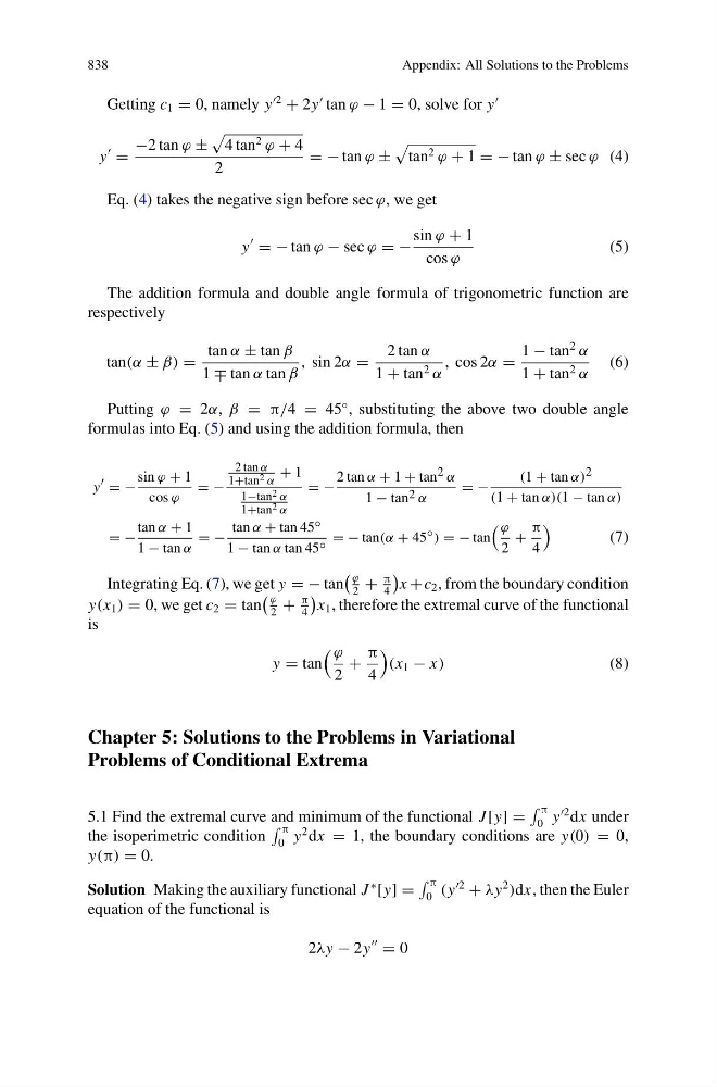
Getting c 1 = 0, namely y
2
+ 2y
tan ϕ − 1 = 0, solve for y
y
=
−2 tan ϕ ±
4 tan 2 ϕ + 4
2
= − tan ϕ ±
tan 2 ϕ + 1 = − tan ϕ ± sec ϕ (4)
Eq. (4) takes the negative sign before sec ϕ, we get
y
= − tan ϕ − sec ϕ = −
sin ϕ + 1
cos ϕ
(5)
The addition formula and double angle formula of trigonometric function are
respectively
tan(α ± β) =
tan α ± tan β
1 ∓ tan α tan β
, sin 2α =
2 tan α
1 + tan 2 α
, cos 2α =
1 − tan
2
α
1 + tan 2 α
(6)
Putting ϕ = 2α, β = π/4 = 45
◦ , substituting the above two double angle
formulas into Eq. (5) and using the addition formula, then
y = −
sin ϕ + 1
cos ϕ
= −
2 tan α
1+tan 2 α
+ 1
1−tan 2 α
1+tan 2 α
= −
2 tan α + 1 + tan 2 α
1 − tan 2 α
= −
(1 + tan α) 2
(1 + tan α)(1 − tan α)
= −
tan α + 1
1 − tan α
= −
tan α + tan 45 ◦
1 − tan α tan 45 ◦ = − tan(α + 45 ◦ ) = − tan
ϕ
2
+
π
4
(7)
Integrating Eq. (7), we get y = − tan
ϕ
2
+
π
4
x +c 2 , from the boundary condition
y(x 1 ) = 0, we get c 2 = tan
ϕ
2
+
π
4
x 1 , therefore the extremal curve of the functional
is
y = tan
ϕ
2
+
π
4
(x 1 − x)
(8)
Chapter 5: Solutions to the Problems in Variational
Problems of Conditional Extrema
5.1 Find the extremal curve and minimum of the functional J [y] =
π
0 y
2 dx under
the isoperimetric condition
π
0 y
2 dx = 1, the boundary conditions are y(0) = 0,
y(π) = 0.
Solution Making the auxiliary functional J
∗
[y] =
π
0 (y
2
+ λy
2
)dx, then the Euler
equation of the functional is
2λy − 2y
= 0
Appendix: All Solutions to the Problems
Getting c 1 = 0, namely y
2
+ 2y
tan ϕ − 1 = 0, solve for y
y
=
−2 tan ϕ ±
4 tan 2 ϕ + 4
2
= − tan ϕ ±
tan 2 ϕ + 1 = − tan ϕ ± sec ϕ (4)
Eq. (4) takes the negative sign before sec ϕ, we get
y
= − tan ϕ − sec ϕ = −
sin ϕ + 1
cos ϕ
(5)
The addition formula and double angle formula of trigonometric function are
respectively
tan(α ± β) =
tan α ± tan β
1 ∓ tan α tan β
, sin 2α =
2 tan α
1 + tan 2 α
, cos 2α =
1 − tan
2
α
1 + tan 2 α
(6)
Putting ϕ = 2α, β = π/4 = 45
◦ , substituting the above two double angle
formulas into Eq. (5) and using the addition formula, then
y = −
sin ϕ + 1
cos ϕ
= −
2 tan α
1+tan 2 α
+ 1
1−tan 2 α
1+tan 2 α
= −
2 tan α + 1 + tan 2 α
1 − tan 2 α
= −
(1 + tan α) 2
(1 + tan α)(1 − tan α)
= −
tan α + 1
1 − tan α
= −
tan α + tan 45 ◦
1 − tan α tan 45 ◦ = − tan(α + 45 ◦ ) = − tan
ϕ
2
+
π
4
(7)
Integrating Eq. (7), we get y = − tan
ϕ
2
+
π
4
x +c 2 , from the boundary condition
y(x 1 ) = 0, we get c 2 = tan
ϕ
2
+
π
4
x 1 , therefore the extremal curve of the functional
is
y = tan
ϕ
2
+
π
4
(x 1 − x)
(8)
Chapter 5: Solutions to the Problems in Variational
Problems of Conditional Extrema
5.1 Find the extremal curve and minimum of the functional J [y] =
π
0 y
2 dx under
the isoperimetric condition
π
0 y
2 dx = 1, the boundary conditions are y(0) = 0,
y(π) = 0.
Solution Making the auxiliary functional J
∗
[y] =
π
0 (y
2
+ λy
2
)dx, then the Euler
equation of the functional is
2λy − 2y
= 0