Appendix: All Solutions to the Problems
771
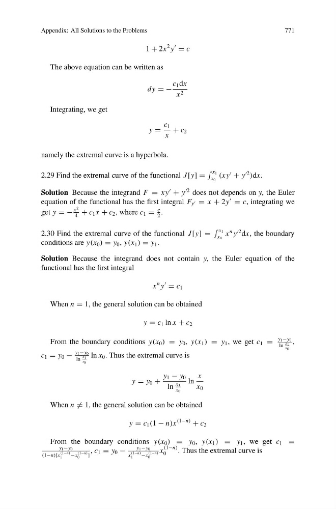
1 + 2x
2 y
= c
The above equation can be written as
dy = −
c 1 dx
x 2
Integrating, we get
y =
c 1
x
+ c 2
namely the extremal curve is a hyperbola.
2.29 Find the extremal curve of the functional J [y] =
x 1
x 0
(x y
+ y
2
)dx.
Solution Because the integrand F = x y
+ y
2 does not depends on y, the Euler
equation of the functional has the first integral F y = x + 2y
= c, integrating we
get y = −
x
2
4
+ c 1 x + c 2 , where c 1 =
c
2
.
2.30 Find the extremal curve of the functional J [y] =
x 1
x 0
x
n y
2 dx, the boundary
conditions are y(x 0 ) = y 0 , y(x 1 ) = y 1 .
Solution Because the integrand does not contain y, the Euler equation of the
functional has the first integral
x
n y
= c 1
When n = 1, the general solution can be obtained
y = c 1 ln x + c 2
From the boundary conditions y(x 0 ) = y 0 , y(x 1 ) = y 1 , we get c 1 =
y 1 −y 0
ln
x 1
x 0
,
c 1 = y 0 −
y 1 −y 0
ln
x 1
x 0
ln x 0 . Thus the extremal curve is
y = y 0 +
y 1 − y 0
ln
x 1
x 0
ln
x
x 0
When n = 1, the general solution can be obtained
y = c 1 (1 − n)x
(1−n)
+ c 2
From the boundary conditions y(x 0 ) = y 0 , y(x 1 ) = y 1 , we get c 1 =
y 1 −y 0
(1−n)[x
(1−n)
1
−x
(1−n)
0
]
, c 1 = y 0 −
y 1 −y 0
x
(1−n)
1
−x
(1−n)
0
x
(1−n)
0
. Thus the extremal curve is