

1.7 Basic Conceptions of Tensors
59
a = (a · e j )e j = a j e j
(1.7.4)
a = (a · e
i )e
i = a
i e
i
(1.7.5)
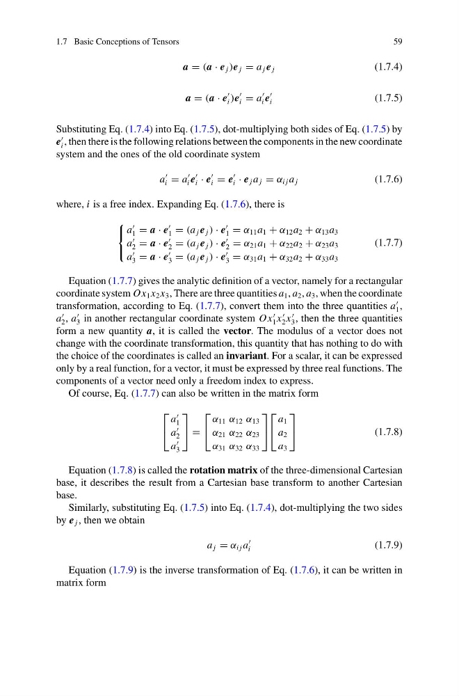
Substituting Eq. (1.7.4) into Eq. (1.7.5), dot-multiplying both sides of Eq. (1.7.5) by
e
i , then there is the following relations between the components in the new coordinate
system and the ones of the old coordinate system
a
i = a
i e
i · e
i = e
i · e j a j = α i j a j
(1.7.6)
where, i is a free index. Expanding Eq. (1.7.6), there is
⎧
⎨
⎩
a
1 = a · e
1 = (a j e j ) · e
1 = α 11 a 1 + α 12 a 2 + α 13 a 3
a
2 = a · e
2 = (a j e j ) · e
2 = α 21 a 1 + α 22 a 2 + α 23 a 3
a
3 = a · e
3 = (a j e j ) · e
3 = α 31 a 1 + α 32 a 2 + α 33 a 3
(1.7.7)
Equation (1.7.7) gives the analytic definition of a vector, namely for a rectangular
coordinate system Ox 1 x 2 x 3 , There are three quantities a 1 , a 2 , a 3 , when the coordinate
transformation, according to Eq. (1.7.7), convert them into the three quantities a
1 ,
a
2 , a
3 in another rectangular coordinate system Ox
1 x
2 x
3 , then the three quantities
form a new quantity a, it is called the vector. The modulus of a vector does not
change with the coordinate transformation, this quantity that has nothing to do with
the choice of the coordinates is called an invariant. For a scalar, it can be expressed
only by a real function, for a vector, it must be expressed by three real functions. The
components of a vector need only a freedom index to express.
Of course, Eq. (1.7.7) can also be written in the matrix form
⎡
⎣
a
1
a
2
a
3
⎤
⎦ =
⎡
⎣
α 11 α 12 α 13
α 21 α 22 α 23
α 31 α 32 α 33
⎤
⎦
⎡
⎣
a 1
a 2
a 3
⎤
⎦
(1.7.8)
Equation (1.7.8) is called the rotation matrix of the three-dimensional Cartesian
base, it describes the result from a Cartesian base transform to another Cartesian
base.
Similarly, substituting Eq. (1.7.5) into Eq. (1.7.4), dot-multiplying the two sides
by e j , then we obtain
a j = α i j a
i
(1.7.9)
Equation (1.7.9) is the inverse transformation of Eq. (1.7.6), it can be written in
matrix form
59
a = (a · e j )e j = a j e j
(1.7.4)
a = (a · e
i )e
i = a
i e
i
(1.7.5)
Substituting Eq. (1.7.4) into Eq. (1.7.5), dot-multiplying both sides of Eq. (1.7.5) by
e
i , then there is the following relations between the components in the new coordinate
system and the ones of the old coordinate system
a
i = a
i e
i · e
i = e
i · e j a j = α i j a j
(1.7.6)
where, i is a free index. Expanding Eq. (1.7.6), there is
⎧
⎨
⎩
a
1 = a · e
1 = (a j e j ) · e
1 = α 11 a 1 + α 12 a 2 + α 13 a 3
a
2 = a · e
2 = (a j e j ) · e
2 = α 21 a 1 + α 22 a 2 + α 23 a 3
a
3 = a · e
3 = (a j e j ) · e
3 = α 31 a 1 + α 32 a 2 + α 33 a 3
(1.7.7)
Equation (1.7.7) gives the analytic definition of a vector, namely for a rectangular
coordinate system Ox 1 x 2 x 3 , There are three quantities a 1 , a 2 , a 3 , when the coordinate
transformation, according to Eq. (1.7.7), convert them into the three quantities a
1 ,
a
2 , a
3 in another rectangular coordinate system Ox
1 x
2 x
3 , then the three quantities
form a new quantity a, it is called the vector. The modulus of a vector does not
change with the coordinate transformation, this quantity that has nothing to do with
the choice of the coordinates is called an invariant. For a scalar, it can be expressed
only by a real function, for a vector, it must be expressed by three real functions. The
components of a vector need only a freedom index to express.
Of course, Eq. (1.7.7) can also be written in the matrix form
⎡
⎣
a
1
a
2
a
3
⎤
⎦ =
⎡
⎣
α 11 α 12 α 13
α 21 α 22 α 23
α 31 α 32 α 33
⎤
⎦
⎡
⎣
a 1
a 2
a 3
⎤
⎦
(1.7.8)
Equation (1.7.8) is called the rotation matrix of the three-dimensional Cartesian
base, it describes the result from a Cartesian base transform to another Cartesian
base.
Similarly, substituting Eq. (1.7.5) into Eq. (1.7.4), dot-multiplying the two sides
by e j , then we obtain
a j = α i j a
i
(1.7.9)
Equation (1.7.9) is the inverse transformation of Eq. (1.7.6), it can be written in
matrix form