10.3 The Euler Equations of Gradient Type Functionals
645
δ J =
V
∂ F
∂u
δu +
∂ F
∂ a
· δa +
∂ F
∂∇∇ · (ua)
· δ∇∇ · (ua)
dV
(2)
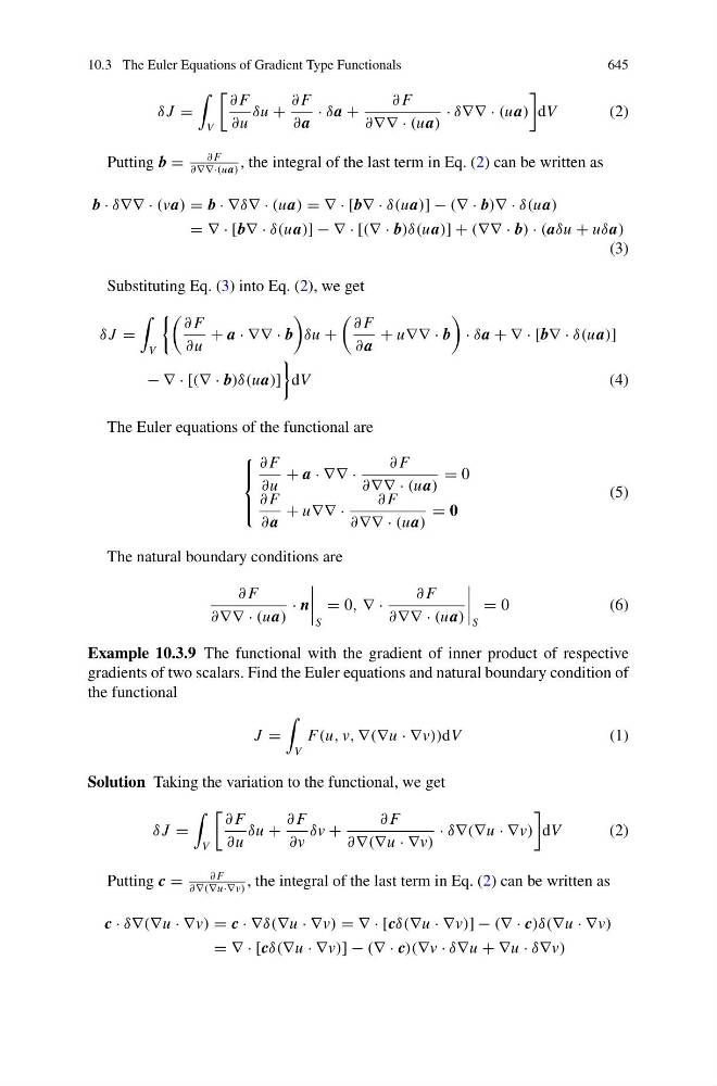
Putting b =
∂ F
∂∇∇·(ua)
, the integral of the last term in Eq. (2) can be written as
b · δ∇∇ · (va) = b · ∇δ∇ · (ua) = ∇ · [b∇ · δ(ua)] − (∇ · b)∇ · δ(ua)
= ∇ · [b∇ · δ(ua)] − ∇ · [(∇ · b)δ(ua)] + (∇∇ · b) · (aδu + uδa)
(3)
Substituting Eq. (3) into Eq. (2), we get
δ J =
V
∂ F
∂u
+ a · ∇∇ · b
δu +
∂ F
∂ a
+ u∇∇ · b
· δa + ∇ · [b∇ · δ(ua)]
− ∇ · [(∇ · b)δ(ua)]
dV
(4)
The Euler equations of the functional are
⎧
⎪ ⎨
⎪ ⎩
∂ F
∂u
+ a · ∇∇ ·
∂ F
∂∇∇ · (ua)
= 0
∂ F
∂ a
+ u∇∇ ·
∂ F
∂∇∇ · (ua)
= 0
(5)
The natural boundary conditions are
∂ F
∂∇∇ · (ua)
· n
S
= 0, ∇ ·
∂ F
∂∇∇ · (ua)
S
= 0
( 6 )
Example 10.3.9 The functional with the gradient of inner product of respective
gradients of two scalars. Find the Euler equations and natural boundary condition of
the functional
J =
V
F(u, v, ∇(∇u · ∇v))dV
(1)
Solution Taking the variation to the functional, we get
δ J =
V
∂ F
∂u
δu +
∂ F
∂v
δv +
∂ F
∂∇(∇u · ∇v)
· δ∇(∇u · ∇v)
dV
(2)
Putting c =
∂ F
∂∇(∇u·∇v)
, the integral of the last term in Eq. (2) can be written as
c · δ∇(∇u · ∇v) = c · ∇δ(∇u · ∇v) = ∇ · [cδ(∇u · ∇v)] − (∇ · c)δ(∇u · ∇v)
= ∇ · [cδ(∇u · ∇v)] − (∇ · c)(∇v · δ∇u + ∇u · δ∇v)