10.2 The Euler Equations of Functionals …
633
⎧
⎪ ⎨
⎪ ⎩
a 1 ψ + 2a 2 |ψ|
2
ψ +
1
2m
e A · (i∇ψ + e Aψ) − ∇ ·
i
2m
(−i∇ψ − e Aψ)
= 0
e
2
m
|ψ|
2 A +
ie
2m
(ψ
∗
∇ψ − ψ∇ψ
∗
) +
∇×B
μ 0
= 0
(2)
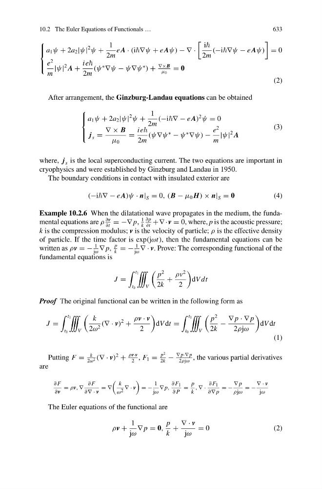
After arrangement, the Ginzburg-Landau equations can be obtained
⎧
⎪ ⎨
⎪ ⎩
a 1 ψ + 2a 2 |ψ|
2
ψ +
1
2m
(−i∇ − e A)
2
ψ = 0
j s =
∇ × B
μ 0
=
ie
2m
(ψ∇ψ
∗
− ψ
∗
∇ψ) −
e
2
m
|ψ|
2 A
(3)
where, j s is the local superconducting current. The two equations are important in
cryophysics and were established by Ginzburg and Landau in 1950.
The boundary conditions in contact with insulated exterior are
(−i∇ − e A)ψ · n| S = 0, (B − μ 0 H) × n| S = 0
(4)
Example 10.2.6 When the dilatational wave propagates in the medium, the fundamental equations are ρ
∂v
∂t
= −∇ p,
1
k
∂ p
∂t
+∇ ·v = 0, where, p is the acoustic pressure;
k is the compression modulus; v is the velocity of particle; ρ is the effective density
of particle. If the time factor is exp(jωt), then the fundamental equations can be
written as ρv = −
1
jω
∇ p,
p
k
= −
1
jω
∇ · v. Prove: The corresponding functional of the
fundamental equations is
J =
t 1
t 0
V
p
2
2k
+
ρv
2
2
dV dt
Proof The original functional can be written in the following form as
J =
t 1
t 0
V
k
2ω 2 (∇ · v)
2
+
ρv · v
2
dV dt =
t 1
t 0
V
p
2
2k
−
∇ p · ∇ p
2ρjω
dV dt
(1)
Putting F =
k
2ω 2 (∇ · v)
2
+
ρv·v
2
, F 1 =
p
2
2k
−
∇ p·∇ p
2ρjω
, the various partial derivatives
are
∂ F
∂v
= ρv, ∇
∂ F
∂∇ · v
= ∇
k
ω 2 ∇ · v
= −
1
jω
∇ p,
∂ F 1
∂ P
=
p
k
, ∇ ·
∂ F 1
∂∇ p
= −
∇ p
ρjω
= −
∇ · v
jω
The Euler equations of the functional are
ρv +
1
jω
∇ p = 0,
p
k
+
∇ · v
jω
= 0
( 2 )