10.2 The Euler Equations of Functionals …
623
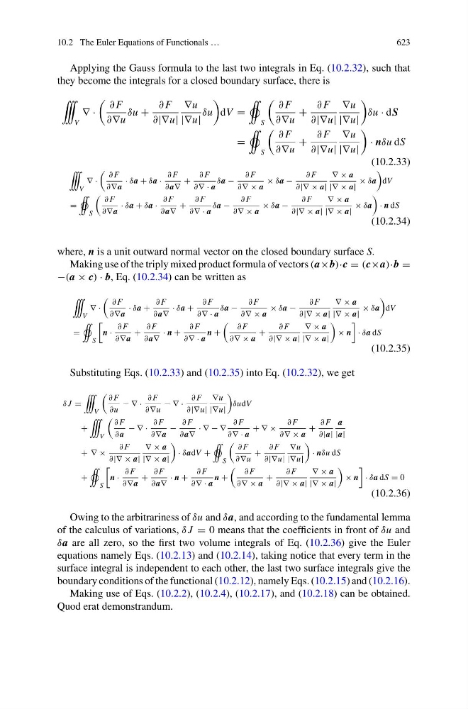
Applying the Gauss formula to the last two integrals in Eq. (10.2.32), such that
they become the integrals for a closed boundary surface, there is
V
∇ ·
∂ F
∂∇u
δu +
∂ F
∂|∇u|
∇u
|∇u|
δu
dV =
S
∂ F
∂∇u
+
∂ F
∂|∇u|
∇u
|∇u|
δu · dS
=
S
∂ F
∂∇u
+
∂ F
∂|∇u|
∇u
|∇u|
· nδu dS
(10.2.33)
V
∇ ·
∂ F
∂∇ a
· δa + δa ·
∂ F
∂ a∇
+
∂ F
∂∇ · a
δa −
∂ F
∂∇ × a
× δa −
∂ F
∂|∇ × a|
∇ × a
|∇ × a|
× δa
dV
=
S
∂ F
∂∇ a
· δa + δa ·
∂ F
∂ a∇
+
∂ F
∂∇ · a
δa −
∂ F
∂∇ × a
× δa −
∂ F
∂|∇ × a|
∇ × a
|∇ × a|
× δa
· n dS
(10.2.34)
where, n is a unit outward normal vector on the closed boundary surface S.
Making use of the triply mixed product formula of vectors (a×b)·c = (c×a)·b =
−(a × c) · b, Eq. (10.2.34) can be written as
V
∇ ·
∂ F
∂∇ a
· δa +
∂ F
∂ a∇
· δa +
∂ F
∂∇ · a
δa −
∂ F
∂∇ × a
× δa −
∂ F
∂|∇ × a|
∇ × a
|∇ × a|
× δa
dV
=
S
n ·
∂ F
∂∇ a
+
∂ F
∂ a∇
· n +
∂ F
∂∇ · a
n +
∂ F
∂∇ × a
+
∂ F
∂|∇ × a|
∇ × a
|∇ × a|
× n
· δa dS
(10.2.35)
Substituting Eqs. (10.2.33) and (10.2.35) into Eq. (10.2.32), we get
δ J =
V
∂ F
∂u
− ∇ ·
∂ F
∂∇u
− ∇ ·
∂ F
∂|∇u|
∇u
|∇u|
δudV
+
V
∂ F
∂ a
− ∇ ·
∂ F
∂∇ a
−
∂ F
∂ a∇
· ∇ − ∇
∂ F
∂∇ · a
+ ∇ ×
∂ F
∂∇ × a
+
∂ F
∂|a|
a
|a|
+ ∇ ×
∂ F
∂|∇ × a|
∇ × a
|∇ × a|
· δadV +
S
∂ F
∂∇u
+
∂ F
∂|∇u|
∇u
|∇u|
· nδu dS
+
S
n ·
∂ F
∂∇ a
+
∂ F
∂ a∇
· n +
∂ F
∂∇ · a
n +
∂ F
∂∇ × a
+
∂ F
∂|∇ × a|
∇ × a
|∇ × a|
× n
· δa dS = 0
(10.2.36)
Owing to the arbitrariness of δu and δa, and according to the fundamental lemma
of the calculus of variations, δ J = 0 means that the coefficients in front of δu and
δa are all zero, so the first two volume integrals of Eq. (10.2.36) give the Euler
equations namely Eqs. (10.2.13) and (10.2.14), taking notice that every term in the
surface integral is independent to each other, the last two surface integrals give the
boundary conditions of the functional (10.2.12), namely Eqs. (10.2.15) and (10.2.16).
Making use of Eqs. (10.2.2), (10.2.4), (10.2.17), and (10.2.18) can be obtained.
Quod erat demonstrandum.