10.1 Basic Properties of the Tensor Inner Product Operations …
617
For every tensor S of order n, if S n
· T = 0, then T = 0. For every symmetrical
tensor S of order n, if S n
· T = 0, then T is an antisymmetrical tensor. For every
antisymmetrical tensor W of order n, if W n
· T = 0, then T is an symmetrical tensor.
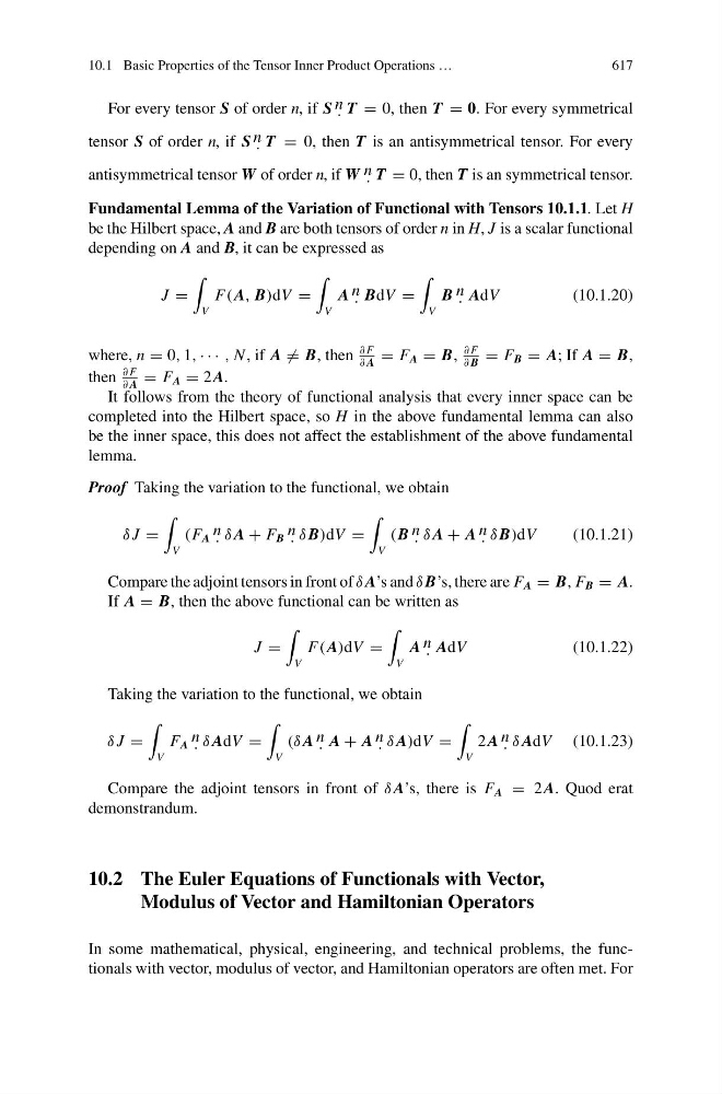
Fundamental Lemma of the Variation of Functional with Tensors 10.1.1. Let H
be the Hilbert space, A and B are both tensors of order n in H, J is a scalar functional
depending on A and B, it can be expressed as
J =
V
F( A, B)dV =
V
A n
· BdV =
V
B n
· AdV
(10.1.20)
where, n = 0, 1, · · · , N , if A = B, then
∂ F
∂ A
= F A = B,
∂ F
∂ B
= F B = A; If A = B,
then
∂ F
∂ A
= F A = 2 A.
It follows from the theory of functional analysis that every inner space can be
completed into the Hilbert space, so H in the above fundamental lemma can also
be the inner space, this does not affect the establishment of the above fundamental
lemma.
Proof Taking the variation to the functional, we obtain
δ J =
V
(F A n
· δ A + F B n
· δ B)dV =
V
(B n
· δ A + A n
· δ B)dV
(10.1.21)
Compare the adjoint tensors in front of δ A’s and δ B’s, there are F A = B, F B = A.
If A = B, then the above functional can be written as
J =
V
F( A)dV =
V
A n
· AdV
(10.1.22)
Taking the variation to the functional, we obtain
δ J =
V
F A n
· δ AdV =
V
(δ A n
· A + A n
· δ A)dV =
V
2 A n
· δ AdV (10.1.23)
Compare the adjoint tensors in front of δ A’s, there is F A = 2 A. Quod erat
demonstrandum.
10.2 The Euler Equations of Functionals with Vector,
Modulus of Vector and Hamiltonian Operators
In some mathematical, physical, engineering, and technical problems, the functionals with vector, modulus of vector, and Hamiltonian operators are often met. For