

586
9 Variational Principles in Mechanics and Their Applications
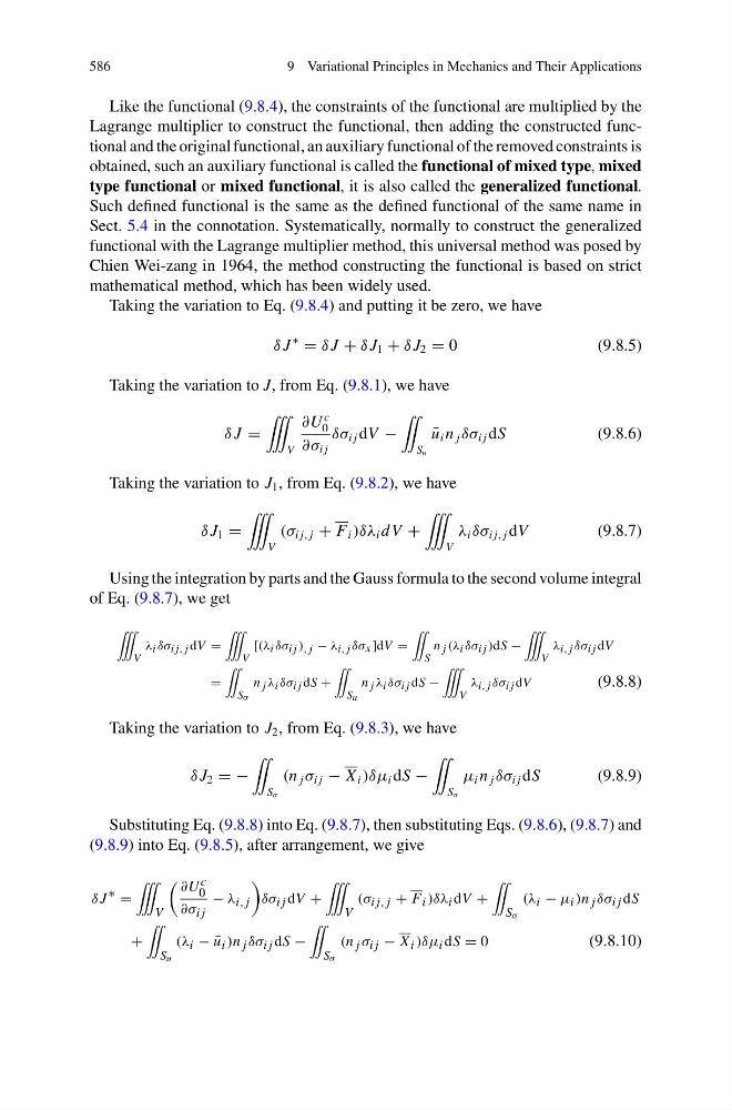
Like the functional (9.8.4), the constraints of the functional are multiplied by the
Lagrange multiplier to construct the functional, then adding the constructed functional and the original functional, an auxiliary functional of the removed constraints is
obtained, such an auxiliary functional is called the functional of mixed type, mixed
type functional or mixed functional, it is also called the generalized functional.
Such defined functional is the same as the defined functional of the same name in
Sect. 5.4 in the connotation. Systematically, normally to construct the generalized
functional with the Lagrange multiplier method, this universal method was posed by
Chien Wei-zang in 1964, the method constructing the functional is based on strict
mathematical method, which has been widely used.
Taking the variation to Eq. (9.8.4) and putting it be zero, we have
δ J
∗
= δ J + δ J 1 + δ J 2 = 0
(9.8.5)
Taking the variation to J, from Eq. (9.8.1), we have
δ J =
˚
V
∂U
c
0
∂σ i j
δσ i j dV −
¨
S u
¯
u i n j δσ i j dS
(9.8.6)
Taking the variation to J 1 , from Eq. (9.8.2), we have
δ J 1 =
˚
V
(σ i j, j + F i )δλ i dV +
˚
V
λ i δσ i j, j dV
(9.8.7)
Using the integration by parts and the Gauss formula to the second volume integral
of Eq. (9.8.7), we get
˚
V
λ i δσ i j, j dV =
˚
V
[(λ i δσ i j ) , j − λ i, j δσ x ]dV =
¨
S
n j (λ i δσ i j )dS −
˚
V
λ i, j δσ i j dV
=
¨
S σ
n j λ i δσ i j dS +
¨
S u
n j λ i δσ i j dS −
˚
V
λ i, j δσ i j dV
(9.8.8)
Taking the variation to J 2 , from Eq. (9.8.3), we have
δ J 2 = −
¨
S σ
(n j σ i j − X i )δμ i dS −
¨
S σ
μ i n j δσ i j dS
(9.8.9)
Substituting Eq. (9.8.8) into Eq. (9.8.7), then substituting Eqs. (9.8.6), (9.8.7) and
(9.8.9) into Eq. (9.8.5), after arrangement, we give
δ J ∗ =
˚
V
∂U c
0
∂σ i j
− λ i, j
δσ i j dV +
˚
V
(σ i j, j + F i )δλ i dV +
¨
S σ
(λ i − μ i )n j δσ i j dS
+
¨
S u
(λ i − ¯
u i )n j δσ i j dS −
¨
S σ
(n j σ i j − X i )δμ i dS = 0
(9.8.10)
9 Variational Principles in Mechanics and Their Applications
Like the functional (9.8.4), the constraints of the functional are multiplied by the
Lagrange multiplier to construct the functional, then adding the constructed functional and the original functional, an auxiliary functional of the removed constraints is
obtained, such an auxiliary functional is called the functional of mixed type, mixed
type functional or mixed functional, it is also called the generalized functional.
Such defined functional is the same as the defined functional of the same name in
Sect. 5.4 in the connotation. Systematically, normally to construct the generalized
functional with the Lagrange multiplier method, this universal method was posed by
Chien Wei-zang in 1964, the method constructing the functional is based on strict
mathematical method, which has been widely used.
Taking the variation to Eq. (9.8.4) and putting it be zero, we have
δ J
∗
= δ J + δ J 1 + δ J 2 = 0
(9.8.5)
Taking the variation to J, from Eq. (9.8.1), we have
δ J =
˚
V
∂U
c
0
∂σ i j
δσ i j dV −
¨
S u
¯
u i n j δσ i j dS
(9.8.6)
Taking the variation to J 1 , from Eq. (9.8.2), we have
δ J 1 =
˚
V
(σ i j, j + F i )δλ i dV +
˚
V
λ i δσ i j, j dV
(9.8.7)
Using the integration by parts and the Gauss formula to the second volume integral
of Eq. (9.8.7), we get
˚
V
λ i δσ i j, j dV =
˚
V
[(λ i δσ i j ) , j − λ i, j δσ x ]dV =
¨
S
n j (λ i δσ i j )dS −
˚
V
λ i, j δσ i j dV
=
¨
S σ
n j λ i δσ i j dS +
¨
S u
n j λ i δσ i j dS −
˚
V
λ i, j δσ i j dV
(9.8.8)
Taking the variation to J 2 , from Eq. (9.8.3), we have
δ J 2 = −
¨
S σ
(n j σ i j − X i )δμ i dS −
¨
S σ
μ i n j δσ i j dS
(9.8.9)
Substituting Eq. (9.8.8) into Eq. (9.8.7), then substituting Eqs. (9.8.6), (9.8.7) and
(9.8.9) into Eq. (9.8.5), after arrangement, we give
δ J ∗ =
˚
V
∂U c
0
∂σ i j
− λ i, j
δσ i j dV +
˚
V
(σ i j, j + F i )δλ i dV +
¨
S σ
(λ i − μ i )n j δσ i j dS
+
¨
S u
(λ i − ¯
u i )n j δσ i j dS −
¨
S σ
(n j σ i j − X i )δμ i dS = 0
(9.8.10)