

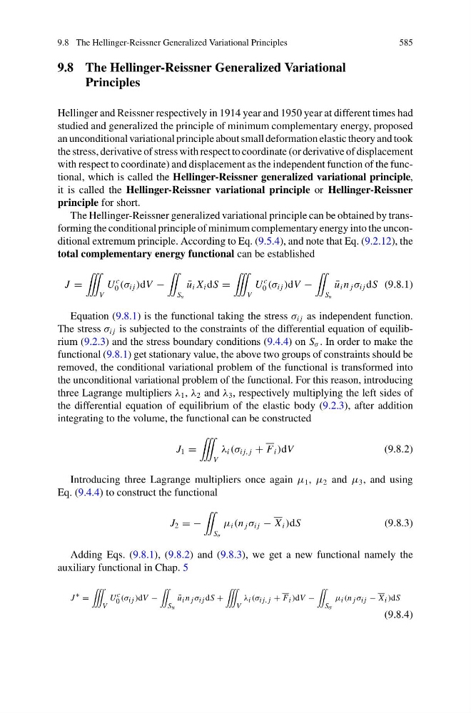
9.8 The Hellinger-Reissner Generalized Variational Principles
585
9.8 The Hellinger-Reissner Generalized Variational
Principles
Hellinger and Reissner respectively in 1914 year and 1950 year at different times had
studied and generalized the principle of minimum complementary energy, proposed
an unconditional variational principle about small deformation elastic theory and took
the stress, derivative of stress with respect to coordinate (or derivative of displacement
with respect to coordinate) and displacement as the independent function of the functional, which is called the Hellinger-Reissner generalized variational principle,
it is called the Hellinger-Reissner variational principle or Hellinger-Reissner
principle for short.
The Hellinger-Reissner generalized variational principle can be obtained by transforming the conditional principle of minimum complementary energy into the unconditional extremum principle. According to Eq. (9.5.4), and note that Eq. (9.2.12), the
total complementary energy functional can be established
J =
˚
V
U
c
0 (σ i j )dV −
¨
S u
¯
u i X i dS =
˚
V
U
c
0 (σ i j )dV −
¨
S u
¯
u i n j σ i j dS (9.8.1)
Equation (9.8.1) is the functional taking the stress σ i j as independent function.
The stress σ i j is subjected to the constraints of the differential equation of equilibrium (9.2.3) and the stress boundary conditions (9.4.4) on S σ . In order to make the
functional (9.8.1) get stationary value, the above two groups of constraints should be
removed, the conditional variational problem of the functional is transformed into
the unconditional variational problem of the functional. For this reason, introducing
three Lagrange multipliers λ 1 , λ 2 and λ 3 , respectively multiplying the left sides of
the differential equation of equilibrium of the elastic body (9.2.3), after addition
integrating to the volume, the functional can be constructed
J 1 =
˚
V
λ i (σ i j, j + F i )dV
(9.8.2)
Introducing three Lagrange multipliers once again μ 1 , μ 2 and μ 3 , and using
Eq. (9.4.4) to construct the functional
J 2 = −
¨
S σ
μ i (n j σ i j − X i )dS
(9.8.3)
Adding Eqs. (9.8.1), (9.8.2) and (9.8.3), we get a new functional namely the
auxiliary functional in Chap. 5
J ∗ =
˚
V
U c
0 (σ i j )dV −
¨
S u
¯
u i n j σ i j dS +
˚
V
λ i (σ i j, j + F i )dV −
¨
S σ
μ i (n j σ i j − X i )dS
(9.8.4)
585
9.8 The Hellinger-Reissner Generalized Variational
Principles
Hellinger and Reissner respectively in 1914 year and 1950 year at different times had
studied and generalized the principle of minimum complementary energy, proposed
an unconditional variational principle about small deformation elastic theory and took
the stress, derivative of stress with respect to coordinate (or derivative of displacement
with respect to coordinate) and displacement as the independent function of the functional, which is called the Hellinger-Reissner generalized variational principle,
it is called the Hellinger-Reissner variational principle or Hellinger-Reissner
principle for short.
The Hellinger-Reissner generalized variational principle can be obtained by transforming the conditional principle of minimum complementary energy into the unconditional extremum principle. According to Eq. (9.5.4), and note that Eq. (9.2.12), the
total complementary energy functional can be established
J =
˚
V
U
c
0 (σ i j )dV −
¨
S u
¯
u i X i dS =
˚
V
U
c
0 (σ i j )dV −
¨
S u
¯
u i n j σ i j dS (9.8.1)
Equation (9.8.1) is the functional taking the stress σ i j as independent function.
The stress σ i j is subjected to the constraints of the differential equation of equilibrium (9.2.3) and the stress boundary conditions (9.4.4) on S σ . In order to make the
functional (9.8.1) get stationary value, the above two groups of constraints should be
removed, the conditional variational problem of the functional is transformed into
the unconditional variational problem of the functional. For this reason, introducing
three Lagrange multipliers λ 1 , λ 2 and λ 3 , respectively multiplying the left sides of
the differential equation of equilibrium of the elastic body (9.2.3), after addition
integrating to the volume, the functional can be constructed
J 1 =
˚
V
λ i (σ i j, j + F i )dV
(9.8.2)
Introducing three Lagrange multipliers once again μ 1 , μ 2 and μ 3 , and using
Eq. (9.4.4) to construct the functional
J 2 = −
¨
S σ
μ i (n j σ i j − X i )dS
(9.8.3)
Adding Eqs. (9.8.1), (9.8.2) and (9.8.3), we get a new functional namely the
auxiliary functional in Chap. 5
J ∗ =
˚
V
U c
0 (σ i j )dV −
¨
S u
¯
u i n j σ i j dS +
˚
V
λ i (σ i j, j + F i )dV −
¨
S σ
μ i (n j σ i j − X i )dS
(9.8.4)