

9.7 The Hamilton’s Canonical Equations
579
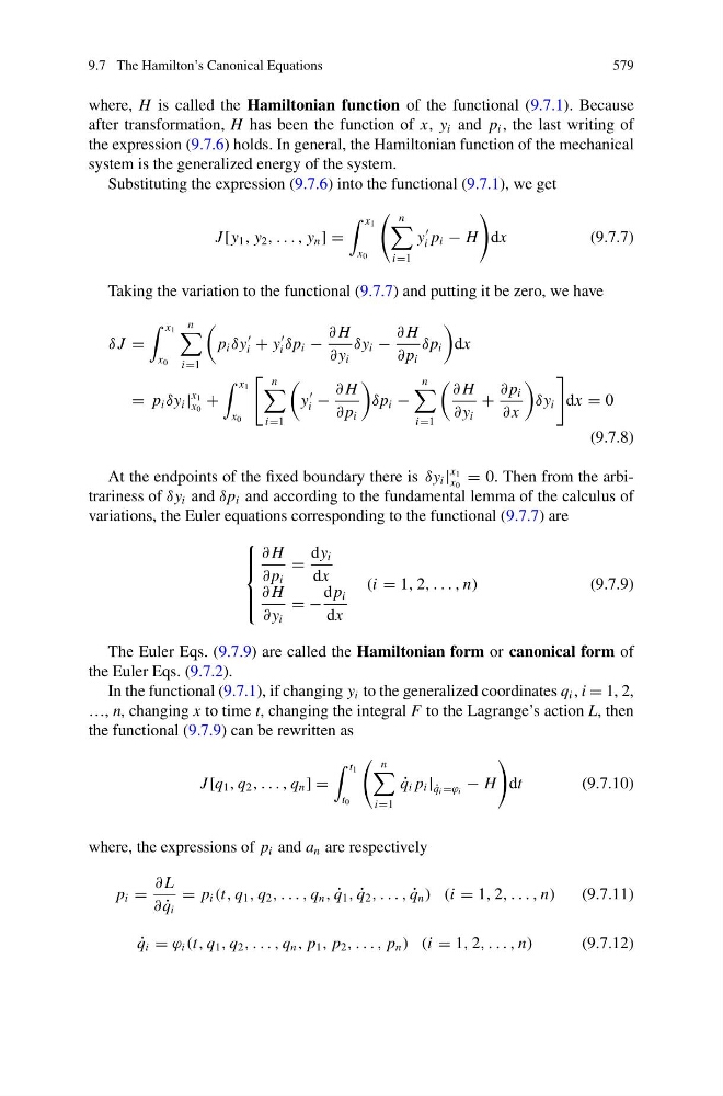
where, H is called the Hamiltonian function of the functional (9.7.1). Because
after transformation, H has been the function of x, y i and p i , the last writing of
the expression (9.7.6) holds. In general, the Hamiltonian function of the mechanical
system is the generalized energy of the system.
Substituting the expression (9.7.6) into the functional (9.7.1), we get
J [y 1 , y 2 , . . . , y n ] =
x 1
x 0
n
i=1
y
i p i − H
dx
(9.7.7)
Taking the variation to the functional (9.7.7) and putting it be zero, we have
δ J =
x 1
x 0
n
i=1
p i δy
i + y
i δp i −
∂ H
∂ y i
δy i −
∂ H
∂ p i
δp i
dx
= p i δy i |
x 1
x 0
+
x 1
x 0
n
i=1
y
i −
∂ H
∂ p i
δp i −
n
i=1
∂ H
∂ y i
+
∂ p i
∂ x
δy i
dx = 0
(9.7.8)
At the endpoints of the fixed boundary there is δy i |
x 1
x 0
= 0. Then from the arbitrariness of δy i and δp i and according to the fundamental lemma of the calculus of
variations, the Euler equations corresponding to the functional (9.7.7) are
⎧
⎪ ⎪ ⎨
⎪ ⎪ ⎩
∂ H
∂ p i
=
dy i
dx
∂ H
∂ y i
= −
d p i
dx
(i = 1, 2, . . . , n)
(9.7.9)
The Euler Eqs. (9.7.9) are called the Hamiltonian form or canonical form of
the Euler Eqs. (9.7.2).
In the functional (9.7.1), if changing y i to the generalized coordinates q i , i = 1, 2,
…, n, changing x to time t, changing the integral F to the Lagrange’s action L, then
the functional (9.7.9) can be rewritten as
J [q 1 , q 2 , . . . , q n ] =
t 1
t 0
n
i=1
˙
q i p i | ˙
q i =ϕ i − H
dt
(9.7.10)
where, the expressions of p i and a n are respectively
p i =
∂ L
∂ ˙
q i
= p i (t, q 1 , q 2 , . . . , q n , ˙
q 1 , ˙
q 2 , . . . , ˙
q n ) (i = 1, 2, . . . , n)
(9.7.11)
˙
q i = ϕ i (t, q 1 , q 2 , . . . , q n , p 1 , p 2 , . . . , p n ) (i = 1, 2, . . . , n)
(9.7.12)
579
where, H is called the Hamiltonian function of the functional (9.7.1). Because
after transformation, H has been the function of x, y i and p i , the last writing of
the expression (9.7.6) holds. In general, the Hamiltonian function of the mechanical
system is the generalized energy of the system.
Substituting the expression (9.7.6) into the functional (9.7.1), we get
J [y 1 , y 2 , . . . , y n ] =
x 1
x 0
n
i=1
y
i p i − H
dx
(9.7.7)
Taking the variation to the functional (9.7.7) and putting it be zero, we have
δ J =
x 1
x 0
n
i=1
p i δy
i + y
i δp i −
∂ H
∂ y i
δy i −
∂ H
∂ p i
δp i
dx
= p i δy i |
x 1
x 0
+
x 1
x 0
n
i=1
y
i −
∂ H
∂ p i
δp i −
n
i=1
∂ H
∂ y i
+
∂ p i
∂ x
δy i
dx = 0
(9.7.8)
At the endpoints of the fixed boundary there is δy i |
x 1
x 0
= 0. Then from the arbitrariness of δy i and δp i and according to the fundamental lemma of the calculus of
variations, the Euler equations corresponding to the functional (9.7.7) are
⎧
⎪ ⎪ ⎨
⎪ ⎪ ⎩
∂ H
∂ p i
=
dy i
dx
∂ H
∂ y i
= −
d p i
dx
(i = 1, 2, . . . , n)
(9.7.9)
The Euler Eqs. (9.7.9) are called the Hamiltonian form or canonical form of
the Euler Eqs. (9.7.2).
In the functional (9.7.1), if changing y i to the generalized coordinates q i , i = 1, 2,
…, n, changing x to time t, changing the integral F to the Lagrange’s action L, then
the functional (9.7.9) can be rewritten as
J [q 1 , q 2 , . . . , q n ] =
t 1
t 0
n
i=1
˙
q i p i | ˙
q i =ϕ i − H
dt
(9.7.10)
where, the expressions of p i and a n are respectively
p i =
∂ L
∂ ˙
q i
= p i (t, q 1 , q 2 , . . . , q n , ˙
q 1 , ˙
q 2 , . . . , ˙
q n ) (i = 1, 2, . . . , n)
(9.7.11)
˙
q i = ϕ i (t, q 1 , q 2 , . . . , q n , p 1 , p 2 , . . . , p n ) (i = 1, 2, . . . , n)
(9.7.12)