

578
9 Variational Principles in Mechanics and Their Applications
It follows from example 9.6.11 to example 9.6.13 that if the base function is
complete, then it can converge to exact solution. The solution results of Problems
9.3 and 9.4 behind this chapter also can prove it.
9.7 The Hamilton’s Canonical Equations
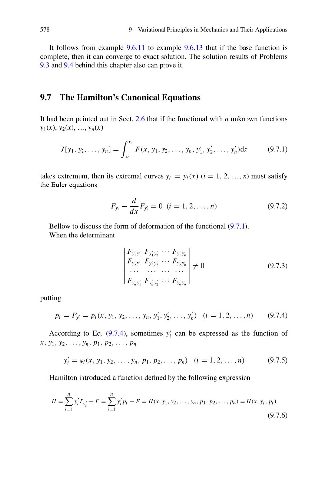
It had been pointed out in Sect. 2.6 that if the functional with n unknown functions
y 1 (x), y 2 (x), …, y n (x)
J [y 1 , y 2 , . . . , y n ] =
x 1
x 0
F(x, y 1 , y 2 , . . . , y n , y
1 , y
2 , . . . , y
n )dx
(9.7.1)
takes extremum, then its extremal curves y i = y i (x) (i = 1, 2, …, n) must satisfy
the Euler equations
F y i −
d
dx
F y
i
= 0 (i = 1, 2, . . . , n)
(9.7.2)
Bellow to discuss the form of deformation of the functional (9.7.1).
When the determinant
F y
1 y
1
F y
1 y
2
· · · F y
1 y
n
F y
2 y
1
F y
2 y
2
· · · F y
2 y
n
· · · · · · · · · · · ·
F y
n y
1
F y
n y
2
· · · F y
n y
n
= 0
(9.7.3)
putting
p i = F y
i
= p i (x, y 1 , y 2 , . . . , y n , y
1 , y
2 , . . . , y
n ) (i = 1, 2, . . . , n)
(9.7.4)
According to Eq. (9.7.4), sometimes y
i can be expressed as the function of
x, y 1 , y 2 , . . . , y n , p 1 , p 2 , . . . , p n
y
i = ϕ i (x, y 1 , y 2 , . . . , y n , p 1 , p 2 , . . . , p n ) (i = 1, 2, . . . , n)
(9.7.5)
Hamilton introduced a function defined by the following expression
H =
n
i=1
y
i F y
i
− F =
n
i=1
y
i p i − F = H (x, y 1 , y 2 , . . . , y n , p 1 , p 2 , . . . , p n ) = H (x, y i , p i )
(9.7.6)
9 Variational Principles in Mechanics and Their Applications
It follows from example 9.6.11 to example 9.6.13 that if the base function is
complete, then it can converge to exact solution. The solution results of Problems
9.3 and 9.4 behind this chapter also can prove it.
9.7 The Hamilton’s Canonical Equations
It had been pointed out in Sect. 2.6 that if the functional with n unknown functions
y 1 (x), y 2 (x), …, y n (x)
J [y 1 , y 2 , . . . , y n ] =
x 1
x 0
F(x, y 1 , y 2 , . . . , y n , y
1 , y
2 , . . . , y
n )dx
(9.7.1)
takes extremum, then its extremal curves y i = y i (x) (i = 1, 2, …, n) must satisfy
the Euler equations
F y i −
d
dx
F y
i
= 0 (i = 1, 2, . . . , n)
(9.7.2)
Bellow to discuss the form of deformation of the functional (9.7.1).
When the determinant
F y
1 y
1
F y
1 y
2
· · · F y
1 y
n
F y
2 y
1
F y
2 y
2
· · · F y
2 y
n
· · · · · · · · · · · ·
F y
n y
1
F y
n y
2
· · · F y
n y
n
= 0
(9.7.3)
putting
p i = F y
i
= p i (x, y 1 , y 2 , . . . , y n , y
1 , y
2 , . . . , y
n ) (i = 1, 2, . . . , n)
(9.7.4)
According to Eq. (9.7.4), sometimes y
i can be expressed as the function of
x, y 1 , y 2 , . . . , y n , p 1 , p 2 , . . . , p n
y
i = ϕ i (x, y 1 , y 2 , . . . , y n , p 1 , p 2 , . . . , p n ) (i = 1, 2, . . . , n)
(9.7.5)
Hamilton introduced a function defined by the following expression
H =
n
i=1
y
i F y
i
− F =
n
i=1
y
i p i − F = H (x, y 1 , y 2 , . . . , y n , p 1 , p 2 , . . . , p n ) = H (x, y i , p i )
(9.7.6)