

572
9 Variational Principles in Mechanics and Their Applications
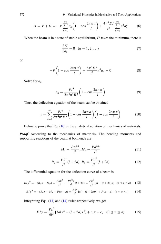
Π = V + U = −P
∞
n=1
a n
1 − cos
2nπ a
l
+
4π
4 E I
l 3
∞
n=1
n
4 a
2
n
(6)
When the beam is in a state of stable equilibrium, Π takes the minimum, there is
∂Π
∂a n
= 0 (n = 1, 2, . . .)
(7)
or
−P
1 − cos
2nπ a
l
+
8π
4 E I
l 3 n
4 a n = 0
( 8 )
Solve for a n
a n =
Pl
3
8π 4 n 4 E I
1 − cos
2nπ a
l
(9)
Thus, the deflection equation of the beam can be obtained
y =
∞
n=1
Pl
3
8π 4 n 4 E I
1 − cos
2nπ a
l
1 − cos
2nπ x
l
(10)
Below to prove that Eq. (10) is the analytical solution of mechanics of materials.
Proof According to the mechanics of materials. The bending moments and
supporting reactions of the beam at both ends are
M a =
Pab
2
l 2 , M b =
Pa
2 b
l 2
(11)
R a =
Pb
2
l 3 (l + 2a), R b =
Pa
2
l 3 (l + 2b)
(12)
The differential equation for the deflection curve of a beam is
E I y = −(R a x − M a ) =
Pab 2
l 2 −
Pb 2 x
l 3 (l + 2a) =
Pb 2
l 3 [al − (l + 2a)x] (0 ≤ x ≤ a) (13)
E I y = −(R a x − M a − P(x − a) =
Pb 2
l 3 [al − (l + 2a)x] + P(x − a) (a ≤ x ≤ l)
(14)
Integrating Eqs. (13) and (14) twice respectively, we get
E I y =
Pb
2
6l 3 [3alx
2
− (l + 2a)x
3
] + c 1 x + c 2 (0 ≤ x ≤ a)
(15)
9 Variational Principles in Mechanics and Their Applications
Π = V + U = −P
∞
n=1
a n
1 − cos
2nπ a
l
+
4π
4 E I
l 3
∞
n=1
n
4 a
2
n
(6)
When the beam is in a state of stable equilibrium, Π takes the minimum, there is
∂Π
∂a n
= 0 (n = 1, 2, . . .)
(7)
or
−P
1 − cos
2nπ a
l
+
8π
4 E I
l 3 n
4 a n = 0
( 8 )
Solve for a n
a n =
Pl
3
8π 4 n 4 E I
1 − cos
2nπ a
l
(9)
Thus, the deflection equation of the beam can be obtained
y =
∞
n=1
Pl
3
8π 4 n 4 E I
1 − cos
2nπ a
l
1 − cos
2nπ x
l
(10)
Below to prove that Eq. (10) is the analytical solution of mechanics of materials.
Proof According to the mechanics of materials. The bending moments and
supporting reactions of the beam at both ends are
M a =
Pab
2
l 2 , M b =
Pa
2 b
l 2
(11)
R a =
Pb
2
l 3 (l + 2a), R b =
Pa
2
l 3 (l + 2b)
(12)
The differential equation for the deflection curve of a beam is
E I y = −(R a x − M a ) =
Pab 2
l 2 −
Pb 2 x
l 3 (l + 2a) =
Pb 2
l 3 [al − (l + 2a)x] (0 ≤ x ≤ a) (13)
E I y = −(R a x − M a − P(x − a) =
Pb 2
l 3 [al − (l + 2a)x] + P(x − a) (a ≤ x ≤ l)
(14)
Integrating Eqs. (13) and (14) twice respectively, we get
E I y =
Pb
2
6l 3 [3alx
2
− (l + 2a)x
3
] + c 1 x + c 2 (0 ≤ x ≤ a)
(15)