

568
9 Variational Principles in Mechanics and Their Applications
O
x
y
l
q
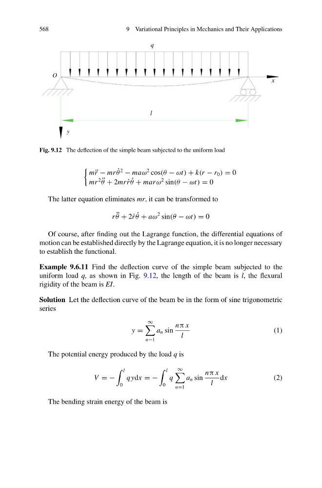
Fig. 9.12 The deflection of the simple beam subjected to the uniform load
m ¨
r − mr ˙
θ
2
− maω
2 cos(θ − ωt) + k(r − r 0 ) = 0
mr
2 ¨
θ + 2mr ˙
r ˙
θ + marω
2 sin(θ − ωt) = 0
The latter equation eliminates mr, it can be transformed to
r ¨
θ + 2˙ r ˙
θ + aω
2 sin(θ − ωt) = 0
Of course, after finding out the Lagrange function, the differential equations of
motion can be established directly by the Lagrange equation, it is no longer necessary
to establish the functional.
Example 9.6.11 Find the deflection curve of the simple beam subjected to the
uniform load q, as shown in Fig. 9.12, the length of the beam is l, the flexural
rigidity of the beam is EI.
Solution Let the deflection curve of the beam be in the form of sine trigonometric
series
y =
∞
n=1
a n sin
nπ x
l
(1)
The potential energy produced by the load q is
V = −
l
0
qydx = −
l
0
q
∞
n=1
a n sin
nπ x
l
dx
(2)
The bending strain energy of the beam is
9 Variational Principles in Mechanics and Their Applications
O
x
y
l
q
Fig. 9.12 The deflection of the simple beam subjected to the uniform load
m ¨
r − mr ˙
θ
2
− maω
2 cos(θ − ωt) + k(r − r 0 ) = 0
mr
2 ¨
θ + 2mr ˙
r ˙
θ + marω
2 sin(θ − ωt) = 0
The latter equation eliminates mr, it can be transformed to
r ¨
θ + 2˙ r ˙
θ + aω
2 sin(θ − ωt) = 0
Of course, after finding out the Lagrange function, the differential equations of
motion can be established directly by the Lagrange equation, it is no longer necessary
to establish the functional.
Example 9.6.11 Find the deflection curve of the simple beam subjected to the
uniform load q, as shown in Fig. 9.12, the length of the beam is l, the flexural
rigidity of the beam is EI.
Solution Let the deflection curve of the beam be in the form of sine trigonometric
series
y =
∞
n=1
a n sin
nπ x
l
(1)
The potential energy produced by the load q is
V = −
l
0
qydx = −
l
0
q
∞
n=1
a n sin
nπ x
l
dx
(2)
The bending strain energy of the beam is