

550
9 Variational Principles in Mechanics and Their Applications
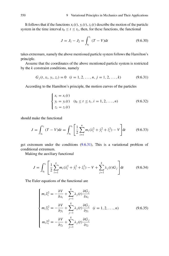
It follows that if the functions x i (t), y i (t), z i (t) describe the motion of the particle
system in the time interval t 0 ≤ t ≤ t 1 , then, for these functions, the functional
J = J 1 − J 2 =
t 1
t 0
(T − V )dt
(9.6.30)
takes extremum, namely the above mentioned particle system follows the Hamilton’s
principle.
Assume that the coordinates of the above mentioned particle system is restricted
by the k constraint conditions, namely
G j (t, x i , y i , z i ) = 0 (i = 1, 2, . . . , n, j = 1, 2, . . . , k)
(9.6.31)
According to the Hamilton’s principle, the motion curves of the particles
⎧
⎪ ⎨
⎪ ⎩
x i = x i (t)
y i = y i (t)
z i = z i (t)
(t 0 ≤ t ≤ t 1 , i = 1, 2, . . . , n)
(9.6.32)
should make the functional
J =
t 1
t 0
(T − V )dt =
t 1
t 0
1
2
n
i=1
m i ( ˙
x
2
i + ˙
y
2
i + ˙
z
2
i ) − V
dt
(9.6.33)
get extremum under the conditions (9.6.31), This is a variational problem of
conditional extremum.
Making the auxiliary functional
J =
t 1
t 0
⎡
⎣ 1
2
n
i=1
m i ( ˙
x
2
i + ˙
y
2
i + ˙
z
2
i ) − V +
k
j=1
λ j (t)G j
⎤
⎦ dt
(9.6.34)
The Euler equations of the functional are
⎧
⎪ ⎪ ⎪ ⎪ ⎪ ⎪ ⎪ ⎪ ⎪ ⎪ ⎪ ⎨
⎪ ⎪ ⎪ ⎪ ⎪ ⎪ ⎪ ⎪ ⎪ ⎪ ⎪ ⎩
m i ¨
x
2
i = −
∂ V
∂ x i
+
k
j=1
λ j (t)
∂G j
∂ x i
m i ¨
y
2
i = −
∂ V
∂ y i
+
k
j=1
λ j (t)
∂G j
∂ y i
m i ¨
z
2
i = −
∂ V
∂z i
+
k
j=1
λ j (t)
∂G j
∂z i
(i = 1, 2, . . . , n)
(9.6.35)
9 Variational Principles in Mechanics and Their Applications
It follows that if the functions x i (t), y i (t), z i (t) describe the motion of the particle
system in the time interval t 0 ≤ t ≤ t 1 , then, for these functions, the functional
J = J 1 − J 2 =
t 1
t 0
(T − V )dt
(9.6.30)
takes extremum, namely the above mentioned particle system follows the Hamilton’s
principle.
Assume that the coordinates of the above mentioned particle system is restricted
by the k constraint conditions, namely
G j (t, x i , y i , z i ) = 0 (i = 1, 2, . . . , n, j = 1, 2, . . . , k)
(9.6.31)
According to the Hamilton’s principle, the motion curves of the particles
⎧
⎪ ⎨
⎪ ⎩
x i = x i (t)
y i = y i (t)
z i = z i (t)
(t 0 ≤ t ≤ t 1 , i = 1, 2, . . . , n)
(9.6.32)
should make the functional
J =
t 1
t 0
(T − V )dt =
t 1
t 0
1
2
n
i=1
m i ( ˙
x
2
i + ˙
y
2
i + ˙
z
2
i ) − V
dt
(9.6.33)
get extremum under the conditions (9.6.31), This is a variational problem of
conditional extremum.
Making the auxiliary functional
J =
t 1
t 0
⎡
⎣ 1
2
n
i=1
m i ( ˙
x
2
i + ˙
y
2
i + ˙
z
2
i ) − V +
k
j=1
λ j (t)G j
⎤
⎦ dt
(9.6.34)
The Euler equations of the functional are
⎧
⎪ ⎪ ⎪ ⎪ ⎪ ⎪ ⎪ ⎪ ⎪ ⎪ ⎪ ⎨
⎪ ⎪ ⎪ ⎪ ⎪ ⎪ ⎪ ⎪ ⎪ ⎪ ⎪ ⎩
m i ¨
x
2
i = −
∂ V
∂ x i
+
k
j=1
λ j (t)
∂G j
∂ x i
m i ¨
y
2
i = −
∂ V
∂ y i
+
k
j=1
λ j (t)
∂G j
∂ y i
m i ¨
z
2
i = −
∂ V
∂z i
+
k
j=1
λ j (t)
∂G j
∂z i
(i = 1, 2, . . . , n)
(9.6.35)