

9.6 The Hamilton Principles and Their Applications
549
⎧
⎪ ⎪ ⎪ ⎪ ⎪ ⎪ ⎨
⎪ ⎪ ⎪ ⎪ ⎪ ⎪ ⎩
m i ¨
x i = F x i = −
∂ V
∂ x i
m i ¨
y i = F y i = −
∂ V
∂ y i
m i ¨
z i = F z i = −
∂ V
∂z i
(i = 1, 2, . . . , n)
(9.6.21)
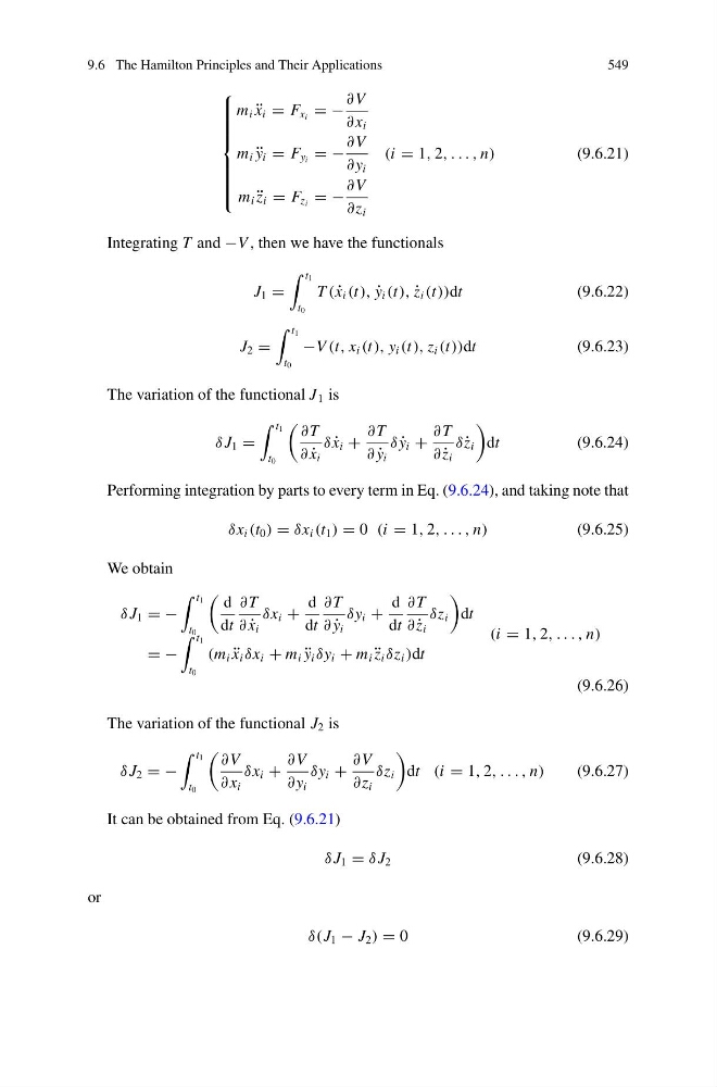
Integrating T and −V , then we have the functionals
J 1 =
t 1
t 0
T ( ˙
x i (t), ˙
y i (t), ˙
z i (t))dt
(9.6.22)
J 2 =
t 1
t 0
−V (t, x i (t), y i (t), z i (t))dt
(9.6.23)
The variation of the functional J 1 is
δ J 1 =
t 1
t 0
∂ T
∂ ˙
x i
δ ˙
x i +
∂ T
∂ ˙
y i
δ ˙
y i +
∂ T
∂ ˙
z i
δ ˙
z i
dt
(9.6.24)
Performing integration by parts to every term in Eq. (9.6.24), and taking note that
δx i (t 0 ) = δx i (t 1 ) = 0 (i = 1, 2, . . . , n)
(9.6.25)
We obtain
δ J 1 = −
t 1
t 0
d
dt
∂ T
∂ ˙
x i
δx i +
d
dt
∂ T
∂ ˙
y i
δy i +
d
dt
∂ T
∂ ˙
z i
δz i
dt
= −
t 1
t 0
(m i ¨
x i δx i + m i ¨
y i δy i + m i ¨
z i δz i )dt
(i = 1, 2, . . . , n)
(9.6.26)
The variation of the functional J 2 is
δ J 2 = −
t 1
t 0
∂ V
∂ x i
δx i +
∂ V
∂ y i
δy i +
∂ V
∂z i
δz i
dt (i = 1, 2, . . . , n)
(9.6.27)
It can be obtained from Eq. (9.6.21)
δ J 1 = δ J 2
(9.6.28)
or
δ(J 1 − J 2 ) = 0
(9.6.29)
549
⎧
⎪ ⎪ ⎪ ⎪ ⎪ ⎪ ⎨
⎪ ⎪ ⎪ ⎪ ⎪ ⎪ ⎩
m i ¨
x i = F x i = −
∂ V
∂ x i
m i ¨
y i = F y i = −
∂ V
∂ y i
m i ¨
z i = F z i = −
∂ V
∂z i
(i = 1, 2, . . . , n)
(9.6.21)
Integrating T and −V , then we have the functionals
J 1 =
t 1
t 0
T ( ˙
x i (t), ˙
y i (t), ˙
z i (t))dt
(9.6.22)
J 2 =
t 1
t 0
−V (t, x i (t), y i (t), z i (t))dt
(9.6.23)
The variation of the functional J 1 is
δ J 1 =
t 1
t 0
∂ T
∂ ˙
x i
δ ˙
x i +
∂ T
∂ ˙
y i
δ ˙
y i +
∂ T
∂ ˙
z i
δ ˙
z i
dt
(9.6.24)
Performing integration by parts to every term in Eq. (9.6.24), and taking note that
δx i (t 0 ) = δx i (t 1 ) = 0 (i = 1, 2, . . . , n)
(9.6.25)
We obtain
δ J 1 = −
t 1
t 0
d
dt
∂ T
∂ ˙
x i
δx i +
d
dt
∂ T
∂ ˙
y i
δy i +
d
dt
∂ T
∂ ˙
z i
δz i
dt
= −
t 1
t 0
(m i ¨
x i δx i + m i ¨
y i δy i + m i ¨
z i δz i )dt
(i = 1, 2, . . . , n)
(9.6.26)
The variation of the functional J 2 is
δ J 2 = −
t 1
t 0
∂ V
∂ x i
δx i +
∂ V
∂ y i
δy i +
∂ V
∂z i
δz i
dt (i = 1, 2, . . . , n)
(9.6.27)
It can be obtained from Eq. (9.6.21)
δ J 1 = δ J 2
(9.6.28)
or
δ(J 1 − J 2 ) = 0
(9.6.29)