

480
8 Direct Methods of Variational Problems
ϕ 2 (x, y) = ϕ 1 (x, y)(x
2
+ y
2
) = (a
2
− x
2
)
2
(b
2
− y
2
)
2
(x
2
+ y
2
)
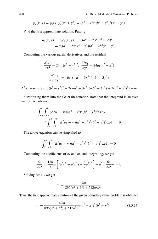
Find the first approximate solution, Putting
u 1 (x, y) = a 1 ϕ 1 (x, y) = a 1 (a
2
− x
2
)
2
(b
2
− y
2
)
2
= a 1 (a
4
− 2a
2 x
2
+ x
4
)(b
4
− 2b
2 y
2
+ y
4
)
Computing the various partial derivatives and the residual
∂
4 u 1
∂ x 4 = 24a 1 (b
2
− y
2
)
2
,
∂
4 u 1
∂ y 4 = 24a 1 (a
2
− x
2
)
∂
4 u 1
∂ x 2 ∂ y 2 = 16a 1 (−a
2
+ 3x
2
)(−b
2
+ 3y
2
)
2 u 1 − m = 8a 1 [3(b
2
− y
2
)
2
+ 2(−a
2
+ 3x
2
)(−b
2
+ 3y
2
) + 3(a
2
− x
2
)
2
] − m
Substituting them into the Galerkin equation, note that the integrand is an even
function, we obtain
a
−a
b
−b
((
2 u 1 − m)(a
2
− x
2
)
2
(b
2
− y
2
)
2 dxdy
= 4
a
0
b
0
((
2 u 1 − m)(a
2
− x
2
)
2
(b
2
− y
2
)
2 dxdy = 0
The above equation can be simplified to
a
0
b
0
((
2 u 1 − m)(a
2
− x
2
)
2
(b
2
− y
2
)
2 dxdy = 0
Computing the coefficients of a 1 and m, and integrating, we get
64
225
×
128
7
a 1
(a
5 b
9
+ a
9 b
5
) +
4
7
a
7 b
7
− a
5 b
5 64
225
m = 0
Solving for a 1 , we get
a 1 =
49m
896(a 4 + b 4 ) + 512a 2 b 2
Thus, the first approximate solution of the given boundary value problem is obtained
u 1 =
49m
896(a 4 + b 4 ) + 512a 2 b 2 (a
2
− x
2
)
2
(b
2
− y
2
)
2
(8.5.24)
8 Direct Methods of Variational Problems
ϕ 2 (x, y) = ϕ 1 (x, y)(x
2
+ y
2
) = (a
2
− x
2
)
2
(b
2
− y
2
)
2
(x
2
+ y
2
)
Find the first approximate solution, Putting
u 1 (x, y) = a 1 ϕ 1 (x, y) = a 1 (a
2
− x
2
)
2
(b
2
− y
2
)
2
= a 1 (a
4
− 2a
2 x
2
+ x
4
)(b
4
− 2b
2 y
2
+ y
4
)
Computing the various partial derivatives and the residual
∂
4 u 1
∂ x 4 = 24a 1 (b
2
− y
2
)
2
,
∂
4 u 1
∂ y 4 = 24a 1 (a
2
− x
2
)
∂
4 u 1
∂ x 2 ∂ y 2 = 16a 1 (−a
2
+ 3x
2
)(−b
2
+ 3y
2
)
2 u 1 − m = 8a 1 [3(b
2
− y
2
)
2
+ 2(−a
2
+ 3x
2
)(−b
2
+ 3y
2
) + 3(a
2
− x
2
)
2
] − m
Substituting them into the Galerkin equation, note that the integrand is an even
function, we obtain
a
−a
b
−b
((
2 u 1 − m)(a
2
− x
2
)
2
(b
2
− y
2
)
2 dxdy
= 4
a
0
b
0
((
2 u 1 − m)(a
2
− x
2
)
2
(b
2
− y
2
)
2 dxdy = 0
The above equation can be simplified to
a
0
b
0
((
2 u 1 − m)(a
2
− x
2
)
2
(b
2
− y
2
)
2 dxdy = 0
Computing the coefficients of a 1 and m, and integrating, we get
64
225
×
128
7
a 1
(a
5 b
9
+ a
9 b
5
) +
4
7
a
7 b
7
− a
5 b
5 64
225
m = 0
Solving for a 1 , we get
a 1 =
49m
896(a 4 + b 4 ) + 512a 2 b 2
Thus, the first approximate solution of the given boundary value problem is obtained
u 1 =
49m
896(a 4 + b 4 ) + 512a 2 b 2 (a
2
− x
2
)
2
(b
2
− y
2
)
2
(8.5.24)