

470
8 Direct Methods of Variational Problems
8.5 The Galerkin Method
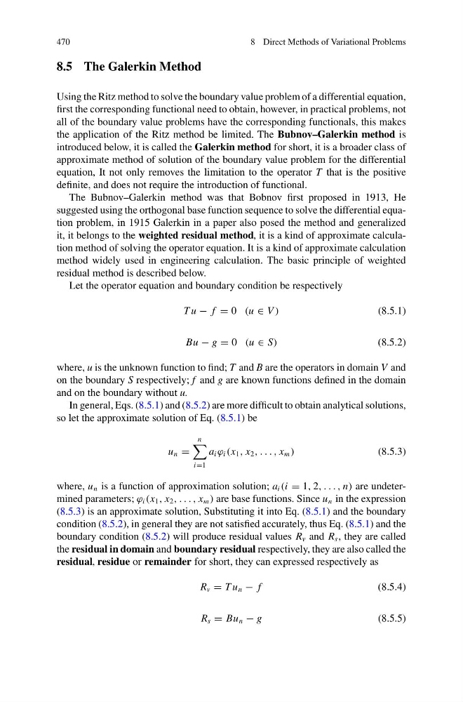
Using the Ritz method to solve the boundary value problem of a differential equation,
first the corresponding functional need to obtain, however, in practical problems, not
all of the boundary value problems have the corresponding functionals, this makes
the application of the Ritz method be limited. The Bubnov–Galerkin method is
introduced below, it is called the Galerkin method for short, it is a broader class of
approximate method of solution of the boundary value problem for the differential
equation, It not only removes the limitation to the operator T that is the positive
definite, and does not require the introduction of functional.
The Bubnov–Galerkin method was that Bobnov first proposed in 1913, He
suggested using the orthogonal base function sequence to solve the differential equation problem, in 1915 Galerkin in a paper also posed the method and generalized
it, it belongs to the weighted residual method, it is a kind of approximate calculation method of solving the operator equation. It is a kind of approximate calculation
method widely used in engineering calculation. The basic principle of weighted
residual method is described below.
Let the operator equation and boundary condition be respectively
T u − f = 0 (u ∈ V )
(8.5.1)
Bu − g = 0 (u ∈ S)
(8.5.2)
where, u is the unknown function to find; T and B are the operators in domain V and
on the boundary S respectively; f and g are known functions defined in the domain
and on the boundary without u.
In general, Eqs. (8.5.1) and (8.5.2) are more difficult to obtain analytical solutions,
so let the approximate solution of Eq. (8.5.1) be
u n =
n
i=1
a i ϕ i (x 1 , x 2 , . . . , x m )
(8.5.3)
where, u n is a function of approximation solution; a i (i = 1, 2, . . . , n) are undetermined parameters; ϕ i (x 1 , x 2 , . . . , x m ) are base functions. Since u n in the expression
(8.5.3) is an approximate solution, Substituting it into Eq. (8.5.1) and the boundary
condition (8.5.2), in general they are not satisfied accurately, thus Eq. (8.5.1) and the
boundary condition (8.5.2) will produce residual values R v and R s , they are called
the residual in domain and boundary residual respectively, they are also called the
residual, residue or remainder for short, they can expressed respectively as
R v = T u n − f
(8.5.4)
R s = Bu n − g
(8.5.5)
8 Direct Methods of Variational Problems
8.5 The Galerkin Method
Using the Ritz method to solve the boundary value problem of a differential equation,
first the corresponding functional need to obtain, however, in practical problems, not
all of the boundary value problems have the corresponding functionals, this makes
the application of the Ritz method be limited. The Bubnov–Galerkin method is
introduced below, it is called the Galerkin method for short, it is a broader class of
approximate method of solution of the boundary value problem for the differential
equation, It not only removes the limitation to the operator T that is the positive
definite, and does not require the introduction of functional.
The Bubnov–Galerkin method was that Bobnov first proposed in 1913, He
suggested using the orthogonal base function sequence to solve the differential equation problem, in 1915 Galerkin in a paper also posed the method and generalized
it, it belongs to the weighted residual method, it is a kind of approximate calculation method of solving the operator equation. It is a kind of approximate calculation
method widely used in engineering calculation. The basic principle of weighted
residual method is described below.
Let the operator equation and boundary condition be respectively
T u − f = 0 (u ∈ V )
(8.5.1)
Bu − g = 0 (u ∈ S)
(8.5.2)
where, u is the unknown function to find; T and B are the operators in domain V and
on the boundary S respectively; f and g are known functions defined in the domain
and on the boundary without u.
In general, Eqs. (8.5.1) and (8.5.2) are more difficult to obtain analytical solutions,
so let the approximate solution of Eq. (8.5.1) be
u n =
n
i=1
a i ϕ i (x 1 , x 2 , . . . , x m )
(8.5.3)
where, u n is a function of approximation solution; a i (i = 1, 2, . . . , n) are undetermined parameters; ϕ i (x 1 , x 2 , . . . , x m ) are base functions. Since u n in the expression
(8.5.3) is an approximate solution, Substituting it into Eq. (8.5.1) and the boundary
condition (8.5.2), in general they are not satisfied accurately, thus Eq. (8.5.1) and the
boundary condition (8.5.2) will produce residual values R v and R s , they are called
the residual in domain and boundary residual respectively, they are also called the
residual, residue or remainder for short, they can expressed respectively as
R v = T u n − f
(8.5.4)
R s = Bu n − g
(8.5.5)