

8.4 The Kantorovich Method
469
where, on the rectangular boundary −a ≤ x ≤ a, −b ≤ y ≤ b, u = 0.
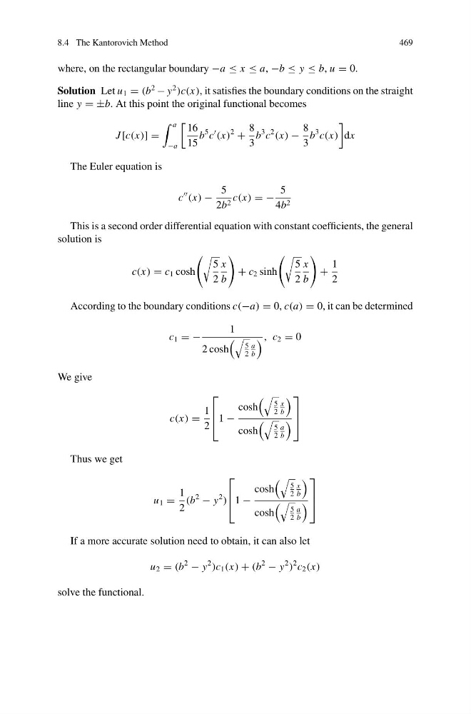
Solution Let u 1 = (b
2
− y
2
)c(x), it satisfies the boundary conditions on the straight
line y = ±b. At this point the original functional becomes
J [c(x)] =
a
−a
16
15
b
5 c
(x)
2
+
8
3
b
3 c
2
(x) −
8
3
b
3 c(x)
dx
The Euler equation is
c
(x) −
5
2b 2 c(x) = −
5
4b 2
This is a second order differential equation with constant coefficients, the general
solution is
c(x) = c 1 cosh
5
2
x
b
+ c 2 sinh
5
2
x
b
+
1
2
According to the boundary conditions c(−a) = 0, c(a) = 0, it can be determined
c 1 = −
1
2 cosh
5
2
a
b
, c 2 = 0
We give
c(x) =
1
2
⎡
⎢
⎣1 −
cosh
5
2
x
b
cosh
5
2
a
b
⎤
⎥
⎦
Thus we get
u 1 =
1
2
(b
2
− y
2
)
⎡
⎢
⎣1 −
cosh
5
2
x
b
cosh
5
2
a
b
⎤
⎥
⎦
If a more accurate solution need to obtain, it can also let
u 2 = (b
2
− y
2
)c 1 (x) + (b
2
− y
2
)
2 c 2 (x)
solve the functional.
469
where, on the rectangular boundary −a ≤ x ≤ a, −b ≤ y ≤ b, u = 0.
Solution Let u 1 = (b
2
− y
2
)c(x), it satisfies the boundary conditions on the straight
line y = ±b. At this point the original functional becomes
J [c(x)] =
a
−a
16
15
b
5 c
(x)
2
+
8
3
b
3 c
2
(x) −
8
3
b
3 c(x)
dx
The Euler equation is
c
(x) −
5
2b 2 c(x) = −
5
4b 2
This is a second order differential equation with constant coefficients, the general
solution is
c(x) = c 1 cosh
5
2
x
b
+ c 2 sinh
5
2
x
b
+
1
2
According to the boundary conditions c(−a) = 0, c(a) = 0, it can be determined
c 1 = −
1
2 cosh
5
2
a
b
, c 2 = 0
We give
c(x) =
1
2
⎡
⎢
⎣1 −
cosh
5
2
x
b
cosh
5
2
a
b
⎤
⎥
⎦
Thus we get
u 1 =
1
2
(b
2
− y
2
)
⎡
⎢
⎣1 −
cosh
5
2
x
b
cosh
5
2
a
b
⎤
⎥
⎦
If a more accurate solution need to obtain, it can also let
u 2 = (b
2
− y
2
)c 1 (x) + (b
2
− y
2
)
2 c 2 (x)
solve the functional.