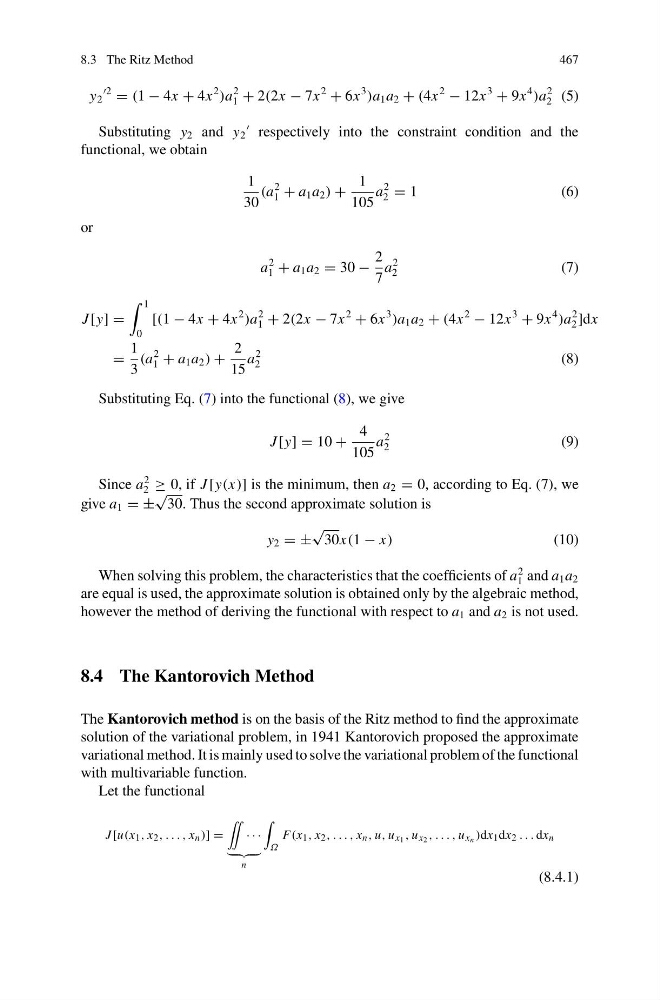
8.3 The Ritz Method
467
y 2
2
= (1 − 4x + 4x
2
)a
2
1 + 2(2x − 7x
2
+ 6x
3
)a 1 a 2 + (4x
2
− 12x
3
+ 9x
4
)a
2
2 (5)
Substituting y 2 and y 2
respectively into the constraint condition and the
functional, we obtain
1
30
(a
2
1 + a 1 a 2 ) +
1
105
a
2
2 = 1
( 6 )
or
a
2
1 + a 1 a 2 = 30 −
2
7
a
2
2
(7)
J [y] =
1
0
[(1 − 4x + 4x
2
)a
2
1 + 2(2x − 7x
2
+ 6x
3
)a 1 a 2 + (4x
2
− 12x
3
+ 9x
4
)a
2
2 ]dx
=
1
3
(a
2
1 + a 1 a 2 ) +
2
15
a
2
2
(8)
Substituting Eq. (7) into the functional (8), we give
J [y] = 10 +
4
105
a
2
2
(9)
Since a
2
2 ≥ 0, if J [y(x)] is the minimum, then a 2 = 0, according to Eq. (7), we
give a 1 = ±
√
30. Thus the second approximate solution is
y 2 = ±
√
30x(1 − x)
(10)
When solving this problem, the characteristics that the coefficients of a
2
1 and a 1 a 2
are equal is used, the approximate solution is obtained only by the algebraic method,
however the method of deriving the functional with respect to a 1 and a 2 is not used.
8.4 The Kantorovich Method
The Kantorovich method is on the basis of the Ritz method to find the approximate
solution of the variational problem, in 1941 Kantorovich proposed the approximate
variational method. It is mainly used to solve the variational problem of the functional
with multivariable function.
Let the functional
J [u(x 1 , x 2 , . . . , x n )] =
¨
· · ·
n
Ω
F(x 1 , x 2 , . . . , x n , u, u x1 , u x2 , . . . , u xn )dx 1 dx 2 . . . dx n
(8.4.1)