

466
8 Direct Methods of Variational Problems
J [v(m)] =
m 0
m 1
α
(aα 2 + b)m
(c + αm)dm =
cα
aα 2 + b
ln
m 0
m 1
+
α
2
(m 0 − m 1 )
aα 2 + b
(3)
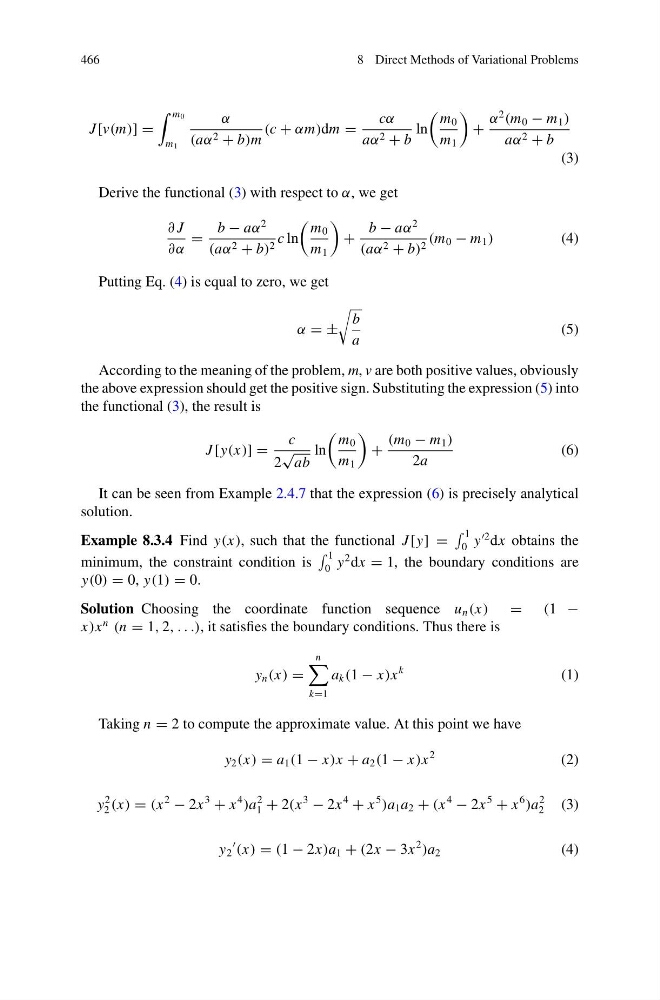
Derive the functional (3) with respect to α, we get
∂ J
∂α
=
b − aα
2
(aα 2 + b) 2 c ln
m 0
m 1
+
b − aα
2
(aα 2 + b) 2 (m 0 − m 1 )
(4)
Putting Eq. (4) is equal to zero, we get
α = ±
b
a
(5)
According to the meaning of the problem, m, v are both positive values, obviously
the above expression should get the positive sign. Substituting the expression (5) into
the functional (3), the result is
J [y(x)] =
c
2
√
ab
ln
m 0
m 1
+
(m 0 − m 1 )
2a
(6)
It can be seen from Example 2.4.7 that the expression (6) is precisely analytical
solution.
Example 8.3.4 Find y(x), such that the functional J [y] =
1
0 y
2 dx obtains the
minimum, the constraint condition is
1
0 y
2 dx = 1, the boundary conditions are
y(0) = 0, y(1) = 0.
Solution Choosing the coordinate function sequence u n (x) = (1 −
x)x
n
(n = 1, 2, . . .), it satisfies the boundary conditions. Thus there is
y n (x) =
n
k=1
a k (1 − x)x
k
(1)
Taking n = 2 to compute the approximate value. At this point we have
y 2 (x) = a 1 (1 − x)x + a 2 (1 − x)x
2
(2)
y
2
2 (x) = (x
2
− 2x
3
+ x
4
)a
2
1 + 2(x
3
− 2x
4
+ x
5
)a 1 a 2 + (x
4
− 2x
5
+ x
6
)a
2
2
(3)
y 2
(x) = (1 − 2x)a 1 + (2x − 3x
2
)a 2
(4)
8 Direct Methods of Variational Problems
J [v(m)] =
m 0
m 1
α
(aα 2 + b)m
(c + αm)dm =
cα
aα 2 + b
ln
m 0
m 1
+
α
2
(m 0 − m 1 )
aα 2 + b
(3)
Derive the functional (3) with respect to α, we get
∂ J
∂α
=
b − aα
2
(aα 2 + b) 2 c ln
m 0
m 1
+
b − aα
2
(aα 2 + b) 2 (m 0 − m 1 )
(4)
Putting Eq. (4) is equal to zero, we get
α = ±
b
a
(5)
According to the meaning of the problem, m, v are both positive values, obviously
the above expression should get the positive sign. Substituting the expression (5) into
the functional (3), the result is
J [y(x)] =
c
2
√
ab
ln
m 0
m 1
+
(m 0 − m 1 )
2a
(6)
It can be seen from Example 2.4.7 that the expression (6) is precisely analytical
solution.
Example 8.3.4 Find y(x), such that the functional J [y] =
1
0 y
2 dx obtains the
minimum, the constraint condition is
1
0 y
2 dx = 1, the boundary conditions are
y(0) = 0, y(1) = 0.
Solution Choosing the coordinate function sequence u n (x) = (1 −
x)x
n
(n = 1, 2, . . .), it satisfies the boundary conditions. Thus there is
y n (x) =
n
k=1
a k (1 − x)x
k
(1)
Taking n = 2 to compute the approximate value. At this point we have
y 2 (x) = a 1 (1 − x)x + a 2 (1 − x)x
2
(2)
y
2
2 (x) = (x
2
− 2x
3
+ x
4
)a
2
1 + 2(x
3
− 2x
4
+ x
5
)a 1 a 2 + (x
4
− 2x
5
+ x
6
)a
2
2
(3)
y 2
(x) = (1 − 2x)a 1 + (2x − 3x
2
)a 2
(4)