

8.3 The Ritz Method
463
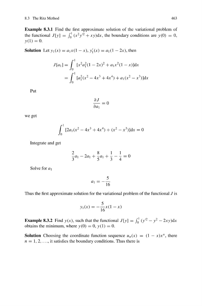
Example 8.3.1 Find the first approximate solution of the variational problem of
the functional J [y] =
1
0 (x
2 y
2
+ x y)dx, the boundary conditions are y(0) = 0,
y(1) = 0.
Solution Let y 1 (x) = a 1 x(1 − x), y
1 (x) = a 1 (1 − 2x), then
J [a 1 ] =
1
0
[x
2 a
2
1 (1 − 2x)
2
+ a 1 x
2
(1 − x)]dx
=
1
0
[a
2
1 (x
2
− 4x
3
+ 4x
4
) + a 1 (x
2
− x
3
)]dx
Put
∂ J
∂a 1
= 0
we get
1
0
[2a 1 (x
2
− 4x
3
+ 4x
4
) + (x
2
− x
3
)]dx = 0
Integrate and get
2
3
a 1 − 2a 1 +
8
5
a 1 +
1
3
−
1
4
= 0
Solve for a 1
a 1 = −
5
16
Thus the first approximate solution for the variational problem of the functional J is
y 1 (x) = −
5
16
x(1 − x)
Example 8.3.2 Find y(x), such that the functional J [y] =
1
0 (y
2
− y
2
− 2x y)dx
obtains the minimum, where y(0) = 0, y(1) = 0.
Solution Choosing the coordinate function sequence u n (x) = (1 − x)x
n , there
n = 1, 2, . . ., it satisfies the boundary conditions. Thus there is
463
Example 8.3.1 Find the first approximate solution of the variational problem of
the functional J [y] =
1
0 (x
2 y
2
+ x y)dx, the boundary conditions are y(0) = 0,
y(1) = 0.
Solution Let y 1 (x) = a 1 x(1 − x), y
1 (x) = a 1 (1 − 2x), then
J [a 1 ] =
1
0
[x
2 a
2
1 (1 − 2x)
2
+ a 1 x
2
(1 − x)]dx
=
1
0
[a
2
1 (x
2
− 4x
3
+ 4x
4
) + a 1 (x
2
− x
3
)]dx
Put
∂ J
∂a 1
= 0
we get
1
0
[2a 1 (x
2
− 4x
3
+ 4x
4
) + (x
2
− x
3
)]dx = 0
Integrate and get
2
3
a 1 − 2a 1 +
8
5
a 1 +
1
3
−
1
4
= 0
Solve for a 1
a 1 = −
5
16
Thus the first approximate solution for the variational problem of the functional J is
y 1 (x) = −
5
16
x(1 − x)
Example 8.3.2 Find y(x), such that the functional J [y] =
1
0 (y
2
− y
2
− 2x y)dx
obtains the minimum, where y(0) = 0, y(1) = 0.
Solution Choosing the coordinate function sequence u n (x) = (1 − x)x
n , there
n = 1, 2, . . ., it satisfies the boundary conditions. Thus there is