

1.3 Fundamentals of the Theory of Field
29
is called the circulation of the vector a along the directing closed curve L.
If the circulation of a vector field is not equal to zero, then it can be thought that
there exists the vortex source producing the field in the vector field. If the circulation
along any closed curve identically vanishes in a vector field, then there can be no
vortex source in the vector field. This kind of vector field is called the irrotational
field, it is called the conservative field in mechanics or physics.
Choosing a point M(x, y, z) in a vector a, to make any micro surface S through
point M, n is the normal vector of the surface at point M, the perimeter of the surface
S is L, its positive direction constitutes the right-handed screw relationship with
n. When S remains the direction of n unchanged at point M and contracts to point
M in arbitrary manner, if there is a limit of ratio between the positive direction
circulation Γ of the vector field a along L and the area S
lim
S→0
Γ
S
= lim
S→0
L a · dL
S
(1.3.79)
then it is called the circulation surface density of the vector field a along n direction
at point M, it is written as rot n a or curl n a, it denotes the projection of the vector
rot a or curl a in the n direction, When using the Hamiltonian operator, it can be
written as (∇ × a) n . Thus, Eq. (1.3.79) can also be written in the following form
rot n a = curl n a = (∇ × a) n = lim
S→0
Γ
S
= lim
S→0
L a · dL
S
(1.3.80)
Obviously the definition of the circulation surface density of point M has nothing
to do with the choice of the coordinate system, it is a quantity that does not to
depend on the choice of the coordinate system, so it is a scalar. It can be seen from
Eq. (1.3.76) that the circulation surface density is the change rate of the circulation
of the directing closed curve to the area surrounded by the closed curve.
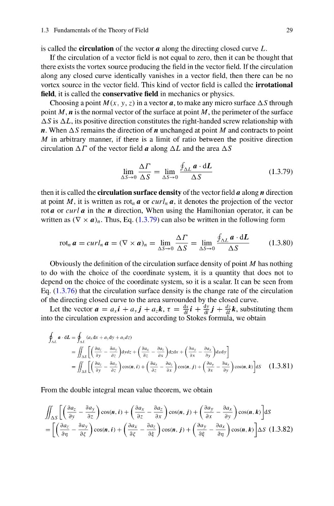
Let the vector a = a x i + a y j + a z k, τ =
dx
dl
i +
dy
dl
j +
dz
dl
k, substituting them
into the circulation expression and according to Stokes formula, we obtain
L
a · dL =
L
(ax dx + ay dy + az dz)
=
¨
S
∂az
∂ y
−
∂ay
∂z
dydz +
∂ax
∂z
−
∂az
∂ x
dzdx +
∂ay
∂ x
−
∂ax
∂ y
dxdy
=
¨
S
∂az
∂ y
−
∂ay
∂z
cos(n, i) +
∂ax
∂z
−
∂az
∂ x
cos(n, j ) +
∂ay
∂ x
−
∂ax
∂ y
cos(n, k)
dS
(1.3.81)
From the double integral mean value theorem, we obtain
¨
S
∂a z
∂ y
−
∂a y
∂z
cos(n, i) +
∂a x
∂z
−
∂a z
∂ x
cos(n, j ) +
∂a y
∂ x
−
∂a x
∂ y
cos(n, k)
dS
=
∂a z
∂η
−
∂a y
∂ζ
cos(n, i) +
∂a x
∂ζ
−
∂a z
∂ξ
cos(n, j ) +
∂a y
∂ξ
−
∂a x
∂η
cos(n, k)
S (1.3.82)
29
is called the circulation of the vector a along the directing closed curve L.
If the circulation of a vector field is not equal to zero, then it can be thought that
there exists the vortex source producing the field in the vector field. If the circulation
along any closed curve identically vanishes in a vector field, then there can be no
vortex source in the vector field. This kind of vector field is called the irrotational
field, it is called the conservative field in mechanics or physics.
Choosing a point M(x, y, z) in a vector a, to make any micro surface S through
point M, n is the normal vector of the surface at point M, the perimeter of the surface
S is L, its positive direction constitutes the right-handed screw relationship with
n. When S remains the direction of n unchanged at point M and contracts to point
M in arbitrary manner, if there is a limit of ratio between the positive direction
circulation Γ of the vector field a along L and the area S
lim
S→0
Γ
S
= lim
S→0
L a · dL
S
(1.3.79)
then it is called the circulation surface density of the vector field a along n direction
at point M, it is written as rot n a or curl n a, it denotes the projection of the vector
rot a or curl a in the n direction, When using the Hamiltonian operator, it can be
written as (∇ × a) n . Thus, Eq. (1.3.79) can also be written in the following form
rot n a = curl n a = (∇ × a) n = lim
S→0
Γ
S
= lim
S→0
L a · dL
S
(1.3.80)
Obviously the definition of the circulation surface density of point M has nothing
to do with the choice of the coordinate system, it is a quantity that does not to
depend on the choice of the coordinate system, so it is a scalar. It can be seen from
Eq. (1.3.76) that the circulation surface density is the change rate of the circulation
of the directing closed curve to the area surrounded by the closed curve.
Let the vector a = a x i + a y j + a z k, τ =
dx
dl
i +
dy
dl
j +
dz
dl
k, substituting them
into the circulation expression and according to Stokes formula, we obtain
L
a · dL =
L
(ax dx + ay dy + az dz)
=
¨
S
∂az
∂ y
−
∂ay
∂z
dydz +
∂ax
∂z
−
∂az
∂ x
dzdx +
∂ay
∂ x
−
∂ax
∂ y
dxdy
=
¨
S
∂az
∂ y
−
∂ay
∂z
cos(n, i) +
∂ax
∂z
−
∂az
∂ x
cos(n, j ) +
∂ay
∂ x
−
∂ax
∂ y
cos(n, k)
dS
(1.3.81)
From the double integral mean value theorem, we obtain
¨
S
∂a z
∂ y
−
∂a y
∂z
cos(n, i) +
∂a x
∂z
−
∂a z
∂ x
cos(n, j ) +
∂a y
∂ x
−
∂a x
∂ y
cos(n, k)
dS
=
∂a z
∂η
−
∂a y
∂ζ
cos(n, i) +
∂a x
∂ζ
−
∂a z
∂ξ
cos(n, j ) +
∂a y
∂ξ
−
∂a x
∂η
cos(n, k)
S (1.3.82)