

436
7 Variational Principles
7.9 The Friedrichs Inequality and Poincaré Inequality
Let G be the bounded domain in the n-dimensional Euclidean space, if the boundary
Γ is sufficiently smooth or piecewise smooth, then such a boundary is called the
Lipschitz boundary or Lipschitzian. The strict definition of this concept is rather
complicated, this definition is just a simple definition. Lipschitz boundaries may be
circles, annuli, triangles, rectangles, spheres and cubes, etc. The bounded domains
most frequently encountered in engineering applications generally belong to the
Lipschitz boundary. For the cases of n = 1, the bounded domain reduced to an
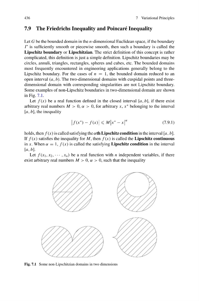
open interval (a, b). The two-dimensional domains with cuspidal points and threedimensional domain with corresponding singularities are not Lipschitz boundary.
Some examples of non-Lipschitz boundaries in two-dimensional domain are shown
in Fig. 7.1.
Let f (x) be a real function defined in the closed interval [a, b], if there exist
arbitrary real numbers M > 0, α > 0, for arbitrary x, x
∗ belonging to the interval
[a, b], the inequality
f (x
∗
) − f (x)
M
x
∗
− x
α
(7.9.1)
holds, then f (x) is called satisfying the αth Lipschitz condition in the interval [a, b].
If f (x) satisfies the inequality for M, then f (x) is called the Lipschitz continuous
in x. When α = 1, f (x) is called the satisfying Lipschitz condition in the interval
[a, b].
Let f (x 1 , x 2 , · · · , x n ) be a real function with n independent variables, if there
exist arbitrary real numbers M > 0, α > 0, such that the inequality
Fig. 7.1 Some non-Lipschitzian domains in two dimensions
7 Variational Principles
7.9 The Friedrichs Inequality and Poincaré Inequality
Let G be the bounded domain in the n-dimensional Euclidean space, if the boundary
Γ is sufficiently smooth or piecewise smooth, then such a boundary is called the
Lipschitz boundary or Lipschitzian. The strict definition of this concept is rather
complicated, this definition is just a simple definition. Lipschitz boundaries may be
circles, annuli, triangles, rectangles, spheres and cubes, etc. The bounded domains
most frequently encountered in engineering applications generally belong to the
Lipschitz boundary. For the cases of n = 1, the bounded domain reduced to an
open interval (a, b). The two-dimensional domains with cuspidal points and threedimensional domain with corresponding singularities are not Lipschitz boundary.
Some examples of non-Lipschitz boundaries in two-dimensional domain are shown
in Fig. 7.1.
Let f (x) be a real function defined in the closed interval [a, b], if there exist
arbitrary real numbers M > 0, α > 0, for arbitrary x, x
∗ belonging to the interval
[a, b], the inequality
f (x
∗
) − f (x)
M
x
∗
− x
α
(7.9.1)
holds, then f (x) is called satisfying the αth Lipschitz condition in the interval [a, b].
If f (x) satisfies the inequality for M, then f (x) is called the Lipschitz continuous
in x. When α = 1, f (x) is called the satisfying Lipschitz condition in the interval
[a, b].
Let f (x 1 , x 2 , · · · , x n ) be a real function with n independent variables, if there
exist arbitrary real numbers M > 0, α > 0, such that the inequality
Fig. 7.1 Some non-Lipschitzian domains in two dimensions