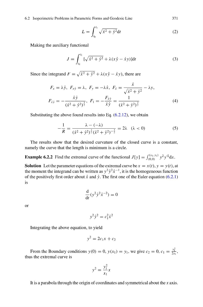
6.2 Isoperimetric Problems in Parametric Forms and Geodesic Line
371
L =
t 1
t 0
˙
x 2 + ˙
y 2 dt
(2)
Making the auxiliary functional
J =
t 1
t 0
[
˙
x 2 + ˙
y 2 + λ(x ˙
y − ˙
x y)]dt
(3)
Since the integrand F =
˙
x 2 + ˙
y 2 + λ(x ˙
y − ˙
x y), there are
F x = λ ˙
y, F x ˙
y = λ, F y = −λ ˙
x, F ˙
x =
˙
x
˙
x 2 + ˙
y 2
− λy,
F ˙
x ˙
y = −
˙
x ˙
y
( ˙
x 2 + ˙
y 2 )
3
2
, F 1 = −
F ˙
x ˙
y
˙
x ˙
y
=
1
( ˙
x 2 + ˙
y 2 )
3
2
(4)
Substituting the above found results into Eq. (6.2.12), we obtain
−
1
R
=
λ − (−λ)
( ˙
x 2 + ˙
y 2 )
3
2 ( ˙
x 2 + ˙
y 2 )
−
3
2
= 2λ (λ < 0)
(5)
The results show that the desired curvature of the closed curve is a constant,
namely the curve that the length is minimum is a circle.
Example 6.2.2 Find the extremal curve of the functional J [y] =
(x 1 ,y 1 )
(0,0)
y
2 y
2 dx.
Solution Let the parameter equations of the extremal curve be x = x(t), y = y(t), at
the moment the integrand can be written as y
2
˙
y
2
˙
x
−1 , it is the homogeneous function
of the positively first order about ˙
x and ˙
y. The first one of the Euler equation (6.2.1)
is
d
dt
(y
2
˙
y
2
˙
x
−2
) = 0
or
y
2
˙
y
2
= c
2
1 ˙
x
2
Integrating the above equation, to yield
y
2
= 2c 1 x + c 2
From the Boundary conditions y(0) = 0, y(x 1 ) = y 1 , we give c 2 = 0, c 1 =
y
2
1
2x 1
,
thus the extremal curve is
y
2
=
y
2
1
x 1
x
It is a parabola through the origin of coordinates and symmetrical about the x axis.