

368
6 Variational Problems in Parametric Forms
=
τ 1
τ 0
F(x(τ ), y(τ ), ˙
x(τ ), ˙
y(τ ))dτ
(6.1.14)
Quod erat demonstrandum.
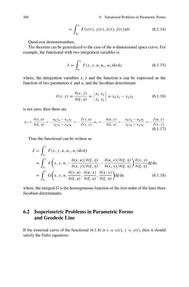
The theorem can be generalized to the case of the n-dimensional space curve. For
example, the functional with two integration variables is
J =
t 1
t 0
F(x, y, u, u x , u y )dxdy
(6.1.15)
where, the integration variables x, y and the function u can be expressed as the
function of two parameters ξ and η, and the Jacobian determinant
J (x, y) =
∂(x, y)
∂(ξ, η)
=
x ξ x η
y ξ y η
= x ξ y η − x η y ξ
(6.1.16)
is not zero, then there are
u x =
∂(y, u)
∂(ξ, η)
= −
u ξ y η − u η y ξ
x ξ y η − x η y ξ
= −
J (y, u)
J (x, y)
, u y = −
∂(u, x)
∂(ξ, η)
= −
u ξ x η − u η x ξ
x ξ y η − x η y ξ
= −
J (u, x)
J (x, y)
(6.1.17)
Thus the functional can be written as
J =
t 1
t 0
F(x, y, u, u x , u y )dxdy
=
t 1
t 0
F
x, y, u, −
∂(y, u)/∂(ξ, η)
∂(x, y)/∂(ξ, η)
, −
∂(u, x)/∂(ξ, η)
∂(x, y)/∂(ξ, η)
∂(x, y)
∂(ξ, η)
dξ dη
=
t 1
t 0
G
x, y, u,
∂(y, u)
∂(ξ, η)
,
∂(u, x)
∂(ξ, η)
,
∂(x, y)
∂(ξ, η)
dξ dη
(6.1.18)
where, the integral G is the homogeneous function of the first order of the later three
Jacobian determinants.
6.2 Isoperimetric Problems in Parametric Forms
and Geodesic Line
If the extremal curve of the functional (6.1.8) is x = x(t), y = y(t), then it should
satisfy the Euler equations
6 Variational Problems in Parametric Forms
=
τ 1
τ 0
F(x(τ ), y(τ ), ˙
x(τ ), ˙
y(τ ))dτ
(6.1.14)
Quod erat demonstrandum.
The theorem can be generalized to the case of the n-dimensional space curve. For
example, the functional with two integration variables is
J =
t 1
t 0
F(x, y, u, u x , u y )dxdy
(6.1.15)
where, the integration variables x, y and the function u can be expressed as the
function of two parameters ξ and η, and the Jacobian determinant
J (x, y) =
∂(x, y)
∂(ξ, η)
=
x ξ x η
y ξ y η
= x ξ y η − x η y ξ
(6.1.16)
is not zero, then there are
u x =
∂(y, u)
∂(ξ, η)
= −
u ξ y η − u η y ξ
x ξ y η − x η y ξ
= −
J (y, u)
J (x, y)
, u y = −
∂(u, x)
∂(ξ, η)
= −
u ξ x η − u η x ξ
x ξ y η − x η y ξ
= −
J (u, x)
J (x, y)
(6.1.17)
Thus the functional can be written as
J =
t 1
t 0
F(x, y, u, u x , u y )dxdy
=
t 1
t 0
F
x, y, u, −
∂(y, u)/∂(ξ, η)
∂(x, y)/∂(ξ, η)
, −
∂(u, x)/∂(ξ, η)
∂(x, y)/∂(ξ, η)
∂(x, y)
∂(ξ, η)
dξ dη
=
t 1
t 0
G
x, y, u,
∂(y, u)
∂(ξ, η)
,
∂(u, x)
∂(ξ, η)
,
∂(x, y)
∂(ξ, η)
dξ dη
(6.1.18)
where, the integral G is the homogeneous function of the first order of the later three
Jacobian determinants.
6.2 Isoperimetric Problems in Parametric Forms
and Geodesic Line
If the extremal curve of the functional (6.1.8) is x = x(t), y = y(t), then it should
satisfy the Euler equations