

5.4 Extremal Problems of Mixed Type Functionals
355
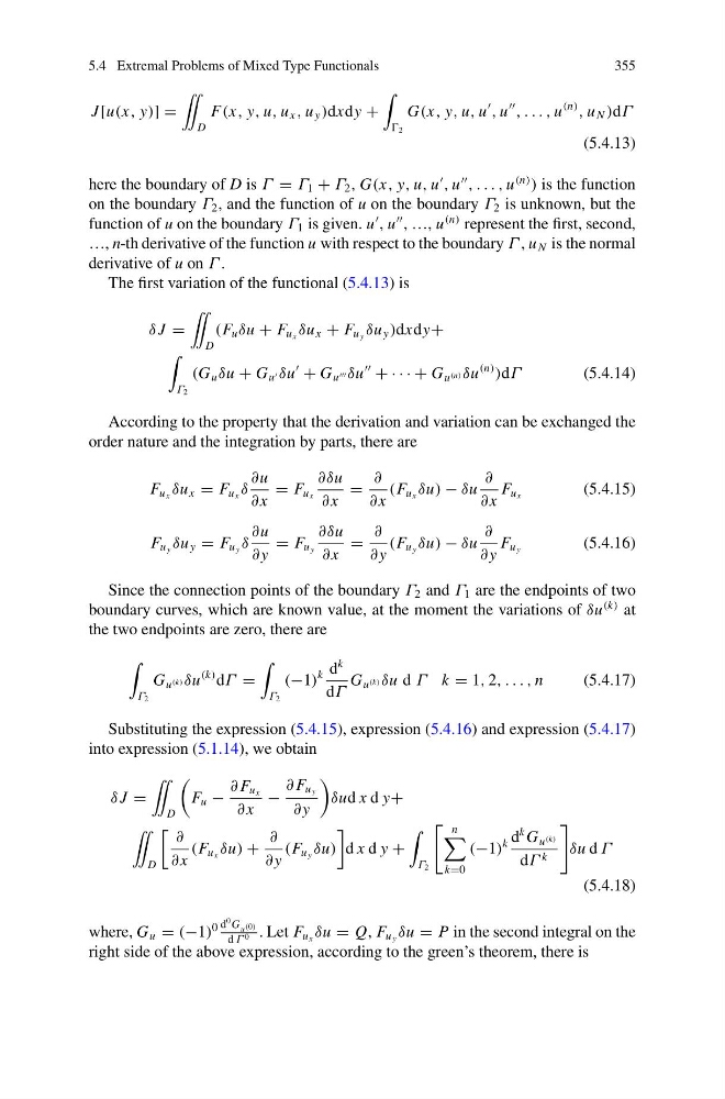
J [u(x, y)] =
¨
D
F(x, y, u, u x , u y )dxdy +
2
G(x, y, u, u
, u
, . . . , u
(n)
, u N )dΓ
(5.4.13)
here the boundary of D is Γ = Γ 1 + Γ 2 , G(x, y, u, u
, u
, . . . , u
(n)
) is the function
on the boundary Γ 2 , and the function of u on the boundary Γ 2 is unknown, but the
function of u on the boundary Γ 1 is given. u
, u
, …, u
(n) represent the first, second,
…, n-th derivative of the function u with respect to the boundary Γ , u N is the normal
derivative of u on Γ .
The first variation of the functional (5.4.13) is
δ J =
¨
D
(F u δu + F u x δu x + F u y δu y )dxdy+
Γ 2
(G u δu + G u δu
+ G u δu
+ · · · + G u (n) δu
(n)
)dΓ
(5.4.14)
According to the property that the derivation and variation can be exchanged the
order nature and the integration by parts, there are
F u x δu x = F u x δ
∂u
∂ x
= F u x
∂δu
∂ x
=
∂
∂ x
(F u x δu) − δu
∂
∂ x
F u x
(5.4.15)
F u y δu y = F u y δ
∂u
∂ y
= F u y
∂δu
∂ x
=
∂
∂ y
(F u y δu) − δu
∂
∂ y
F u y
(5.4.16)
Since the connection points of the boundary Γ 2 and Γ 1 are the endpoints of two
boundary curves, which are known value, at the moment the variations of δu
(k) at
the two endpoints are zero, there are
Γ 2
G u (k) δu
(k) dΓ =
Γ 2
(−1)
k d
k
dΓ
G u (k) δu d Γ k = 1, 2, . . . , n
(5.4.17)
Substituting the expression (5.4.15), expression (5.4.16) and expression (5.4.17)
into expression (5.1.14), we obtain
δ J =
¨
D
F u −
∂ F u x
∂ x
−
∂ F u y
∂ y
δud x d y+
¨
D
∂
∂ x
(F u x δu) +
∂
∂ y
(F u y δu)
d x d y +
Γ 2
n
k=0
(−1)
k d
k G u (k)
dΓ k
δu d Γ
(5.4.18)
where, G u = (−1)
0 d
0 G u (0)
d Γ 0 . Let F u x δu = Q, F u y δu = P in the second integral on the
right side of the above expression, according to the green’s theorem, there is
355
J [u(x, y)] =
¨
D
F(x, y, u, u x , u y )dxdy +
2
G(x, y, u, u
, u
, . . . , u
(n)
, u N )dΓ
(5.4.13)
here the boundary of D is Γ = Γ 1 + Γ 2 , G(x, y, u, u
, u
, . . . , u
(n)
) is the function
on the boundary Γ 2 , and the function of u on the boundary Γ 2 is unknown, but the
function of u on the boundary Γ 1 is given. u
, u
, …, u
(n) represent the first, second,
…, n-th derivative of the function u with respect to the boundary Γ , u N is the normal
derivative of u on Γ .
The first variation of the functional (5.4.13) is
δ J =
¨
D
(F u δu + F u x δu x + F u y δu y )dxdy+
Γ 2
(G u δu + G u δu
+ G u δu
+ · · · + G u (n) δu
(n)
)dΓ
(5.4.14)
According to the property that the derivation and variation can be exchanged the
order nature and the integration by parts, there are
F u x δu x = F u x δ
∂u
∂ x
= F u x
∂δu
∂ x
=
∂
∂ x
(F u x δu) − δu
∂
∂ x
F u x
(5.4.15)
F u y δu y = F u y δ
∂u
∂ y
= F u y
∂δu
∂ x
=
∂
∂ y
(F u y δu) − δu
∂
∂ y
F u y
(5.4.16)
Since the connection points of the boundary Γ 2 and Γ 1 are the endpoints of two
boundary curves, which are known value, at the moment the variations of δu
(k) at
the two endpoints are zero, there are
Γ 2
G u (k) δu
(k) dΓ =
Γ 2
(−1)
k d
k
dΓ
G u (k) δu d Γ k = 1, 2, . . . , n
(5.4.17)
Substituting the expression (5.4.15), expression (5.4.16) and expression (5.4.17)
into expression (5.1.14), we obtain
δ J =
¨
D
F u −
∂ F u x
∂ x
−
∂ F u y
∂ y
δud x d y+
¨
D
∂
∂ x
(F u x δu) +
∂
∂ y
(F u y δu)
d x d y +
Γ 2
n
k=0
(−1)
k d
k G u (k)
dΓ k
δu d Γ
(5.4.18)
where, G u = (−1)
0 d
0 G u (0)
d Γ 0 . Let F u x δu = Q, F u y δu = P in the second integral on the
right side of the above expression, according to the green’s theorem, there is