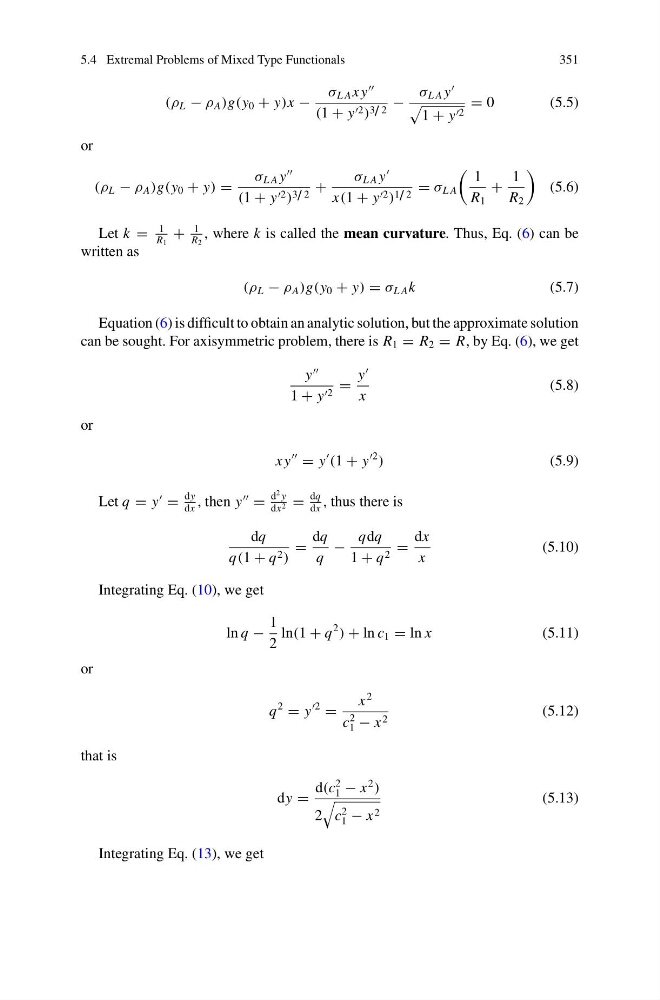
5.4 Extremal Problems of Mixed Type Functionals
351
(ρ L − ρ A )g(y 0 + y)x −
σ L A x y
(1 + y 2 ) 3 / 2 −
σ L A y
1 + y 2
= 0
(5.5)
or
(ρ L − ρ A )g(y 0 + y) =
σ L A y
(1 + y 2 ) 3 / 2 +
σ L A y
x(1 + y 2 ) 1 / 2 = σ L A
1
R 1
+
1
R 2
(5.6)
Let k =
1
R 1
+
1
R 2
, where k is called the mean curvature. Thus, Eq. (6) can be
written as
(ρ L − ρ A )g(y 0 + y) = σ L A k
(5.7)
Equation (6) is difficult to obtain an analytic solution, but the approximate solution
can be sought. For axisymmetric problem, there is R 1 = R 2 = R, by Eq. (6), we get
y
1 + y 2 =
y
x
(5.8)
or
x y
= y
(1 + y
2
)
(5.9)
Let q = y
=
dy
dx
, then y
=
d
2 y
dx 2 =
dq
dx
, thus there is
dq
q(1 + q 2 )
=
dq
q
−
qdq
1 + q 2 =
dx
x
(5.10)
Integrating Eq. (10), we get
ln q −
1
2
ln(1 + q
2
) + ln c 1 = ln x
(5.11)
or
q
2
= y
2
=
x
2
c
2
1 − x 2
(5.12)
that is
dy =
d(c
2
1 − x
2
)
2
c
2
1 − x 2
(5.13)
Integrating Eq. (13), we get