

332
5 Variational Problems of Conditional Extrema
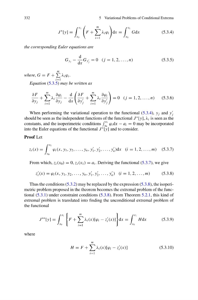
J
∗
[y] =
x 1
x 0
F +
m
i=1
λ i ϕ i
dx =
x 1
x 0
Gdx
(5.3.4)
the corresponding Euler equations are
G y j −
d
dx
G y
j
= 0 ( j = 1, 2, . . . , n)
(5.3.5)
where, G = F +
m
i=1
λ i ϕ i .
Equation (5.3.5) may be written as
∂ F
∂ y j
+
m
i=1
λ i
∂ϕ i
∂ y j
−
d
dx
∂ F
∂ y
j
+
m
i=1
λ i
∂ϕ i
∂ y
j
= 0 ( j = 1, 2, . . . , n)
(5.3.6)
When performing the variational operation to the functional (5.3.4), y j and y
j
should be seen as the independent functions of the functional J
∗
[y], λ i is seen as the
constants, and the isoperimetric conditions
x 1
x 0
ϕ i dx − a i = 0 may be incorporated
into the Euler equations of the functional J
∗
[y] and to consider.
Proof Let
z i (x) =
x 1
x 0
ϕ i (x, y 1 , y 2 , . . . , y n , y
1 , y
2 , . . . , y
n )dx (i = 1, 2, . . . , m) (5.3.7)
From which, z i (x 0 ) = 0, z i (x 1 ) = a i . Deriving the functional (5.3.7), we give
z
i (x) = ϕ i (x, y 1 , y 2 , . . . , y n , y
1 , y
2 , . . . , y
n ) (i = 1, 2, . . . , m)
(5.3.8)
Thus the conditions (5.3.2) may be replaced by the expression (5.3.8), the isoperimetric problem proposed in the theorem becomes the extremal problem of the functional (5.3.1) under constraint conditions (5.3.8). From Theorem 5.2.1, this kind of
extremal problem is translated into finding the unconditional extremal problem of
the functional
J
∗∗
[y] =
x 1
x 0
F +
m
i=1
λ i (x)[ϕ i − z
i (x)]
dx =
x 1
x 0
H dx
(5.3.9)
where
H = F +
m
i=1
λ i (x)[ϕ i − z
i (x)]
(5.3.10)
5 Variational Problems of Conditional Extrema
J
∗
[y] =
x 1
x 0
F +
m
i=1
λ i ϕ i
dx =
x 1
x 0
Gdx
(5.3.4)
the corresponding Euler equations are
G y j −
d
dx
G y
j
= 0 ( j = 1, 2, . . . , n)
(5.3.5)
where, G = F +
m
i=1
λ i ϕ i .
Equation (5.3.5) may be written as
∂ F
∂ y j
+
m
i=1
λ i
∂ϕ i
∂ y j
−
d
dx
∂ F
∂ y
j
+
m
i=1
λ i
∂ϕ i
∂ y
j
= 0 ( j = 1, 2, . . . , n)
(5.3.6)
When performing the variational operation to the functional (5.3.4), y j and y
j
should be seen as the independent functions of the functional J
∗
[y], λ i is seen as the
constants, and the isoperimetric conditions
x 1
x 0
ϕ i dx − a i = 0 may be incorporated
into the Euler equations of the functional J
∗
[y] and to consider.
Proof Let
z i (x) =
x 1
x 0
ϕ i (x, y 1 , y 2 , . . . , y n , y
1 , y
2 , . . . , y
n )dx (i = 1, 2, . . . , m) (5.3.7)
From which, z i (x 0 ) = 0, z i (x 1 ) = a i . Deriving the functional (5.3.7), we give
z
i (x) = ϕ i (x, y 1 , y 2 , . . . , y n , y
1 , y
2 , . . . , y
n ) (i = 1, 2, . . . , m)
(5.3.8)
Thus the conditions (5.3.2) may be replaced by the expression (5.3.8), the isoperimetric problem proposed in the theorem becomes the extremal problem of the functional (5.3.1) under constraint conditions (5.3.8). From Theorem 5.2.1, this kind of
extremal problem is translated into finding the unconditional extremal problem of
the functional
J
∗∗
[y] =
x 1
x 0
F +
m
i=1
λ i (x)[ϕ i − z
i (x)]
dx =
x 1
x 0
H dx
(5.3.9)
where
H = F +
m
i=1
λ i (x)[ϕ i − z
i (x)]
(5.3.10)