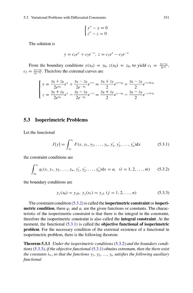
5.2 Variational Problems with Differential Constraints
331
y
− y = 0
z
− z = 0
The solution is
y = c 1 e
x
+ c 2 e
−x
, z = c 1 e
x
− c 2 e
−x
From the boundary conditions y(x 0 ) = y 0 , z(x 0 ) = z 0 , to yield c 1 =
y 0 +z 0
2e x 0 ,
c 2 =
y 0 −z 0
2e −x 0 . Therefore the extremal curves are
⎧
⎪ ⎨
⎪ ⎩
y =
y 0 + z 0
2e x 0
e
x
+
y 0 − z 0
2e −x 0
e
−x
=
y 0 + z 0
2
e
x−x 0 +
y 0 − z 0
2
e
−x+x 0
z =
y 0 + z 0
2e x 0
e
x
−
y 0 − z 0
2e −x 0
e
−x
=
y 0 + z 0
2
e
x−x 0 −
y 0 − z 0
2
e
−x+x 0
5.3 Isoperimetric Problems
Let the functional
J [y] =
x 1
x 0
F(x, y 1 , y 2 , . . . , y n , y
1 , y
2 , . . . , y
n )dx
(5.3.1)
the constraint conditions are
x 1
x 0
ϕ i (x, y 1 , y 2 , . . . , y n , y
1 , y
2 , . . . , y
n )dx = a i (i = 1, 2, . . . , m)
(5.3.2)
the boundary conditions are
y j (x 0 ) = y j0 , y j (x 1 ) = y j1 ( j = 1, 2, . . . , n)
(5.3.3)
The constraint condition (5.3.2) is called the isoperimetric constraint or isoperimetric condition, there ϕ i and a i are the given functions or constants. The characteristic of the isoperimetric constraint is that there is the integral in the constraint,
therefore the isoperimetric constraint is also called the integral constraint. At the
moment, the functional (5.3.1) is called the objective functional of isoperimetric
problem. For the necessary condition of the extremal existence of a functional in
isoperimetric problem, there is the following theorem:
Theorem 5.3.1 Under the isoperimetric conditions (5.3.2) and the boundary conditions (5.3.3), if the objective functional (5.3.1) obtains extremum, then the there exist
the constants λ i , so that the functions y 1 , y 2 , …, y n satisfies the following auxiliary
functional