

5.1 Variational Problems with Holonomic Constraints
325
⎧
⎪ ⎪ ⎨
⎪ ⎪ ⎩
−
d
dx
y
1 + y 2 + z 2
= 0
2λ(x) −
d
dx
z
1 + y 2 + z 2
= 0
(5.3)
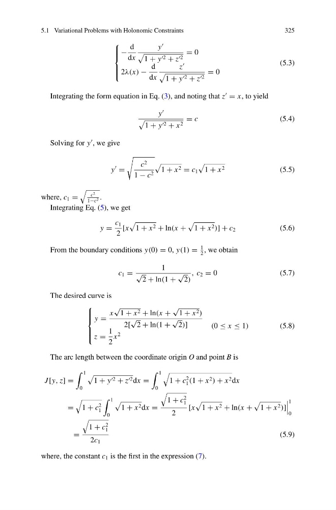
Integrating the form equation in Eq. (3), and noting that z
= x, to yield
y
1 + y 2 + x 2
= c
(5.4)
Solving for y
, we give
y
=
c 2
1 − c 2
1 + x 2 = c 1
1 + x 2
(5.5)
where, c 1 =
c 2
1−c 2 .
Integrating Eq. (5), we get
y =
c 1
2
[x
1 + x 2 + ln(x +
1 + x 2 )] + c 2
(5.6)
From the boundary conditions y(0) = 0, y(1) =
1
2
, we obtain
c 1 =
1
√
2 + ln(1 +
√
2)
, c 2 = 0
(5.7)
The desired curve is
⎧
⎪ ⎪ ⎨
⎪ ⎪ ⎩
y =
x
√
1 + x 2 + ln(x +
√
1 + x 2 )
2[
√
2 + ln(1 +
√
2)]
z =
1
2
x
2
(0 ≤ x ≤ 1)
(5.8)
The arc length between the coordinate origin O and point B is
J [y, z] =
1
0
1 + y 2 + z 2 dx =
1
0
1 + c
2
1 (1 + x 2 ) + x 2 dx
=
1 + c
2
1
1
0
1 + x 2 dx =
1 + c
2
1
2
[x
1 + x 2 + ln(x +
1 + x 2 )]
1
0
=
1 + c
2
1
2c 1
(5.9)
where, the constant c 1 is the first in the expression (7).
325
⎧
⎪ ⎪ ⎨
⎪ ⎪ ⎩
−
d
dx
y
1 + y 2 + z 2
= 0
2λ(x) −
d
dx
z
1 + y 2 + z 2
= 0
(5.3)
Integrating the form equation in Eq. (3), and noting that z
= x, to yield
y
1 + y 2 + x 2
= c
(5.4)
Solving for y
, we give
y
=
c 2
1 − c 2
1 + x 2 = c 1
1 + x 2
(5.5)
where, c 1 =
c 2
1−c 2 .
Integrating Eq. (5), we get
y =
c 1
2
[x
1 + x 2 + ln(x +
1 + x 2 )] + c 2
(5.6)
From the boundary conditions y(0) = 0, y(1) =
1
2
, we obtain
c 1 =
1
√
2 + ln(1 +
√
2)
, c 2 = 0
(5.7)
The desired curve is
⎧
⎪ ⎪ ⎨
⎪ ⎪ ⎩
y =
x
√
1 + x 2 + ln(x +
√
1 + x 2 )
2[
√
2 + ln(1 +
√
2)]
z =
1
2
x
2
(0 ≤ x ≤ 1)
(5.8)
The arc length between the coordinate origin O and point B is
J [y, z] =
1
0
1 + y 2 + z 2 dx =
1
0
1 + c
2
1 (1 + x 2 ) + x 2 dx
=
1 + c
2
1
1
0
1 + x 2 dx =
1 + c
2
1
2
[x
1 + x 2 + ln(x +
1 + x 2 )]
1
0
=
1 + c
2
1
2c 1
(5.9)
where, the constant c 1 is the first in the expression (7).