

306
4 Problems with Variable Boundaries
J [y(x)] =
x 1
x 0
F(x, y, y
)dx =
x M
x 0
F(x, y, y
)dx
+
x N
x M
F(x, ϕ, ϕ
)dx +
x 1
x N
F(x, y, y
)dx
(4.6.14)
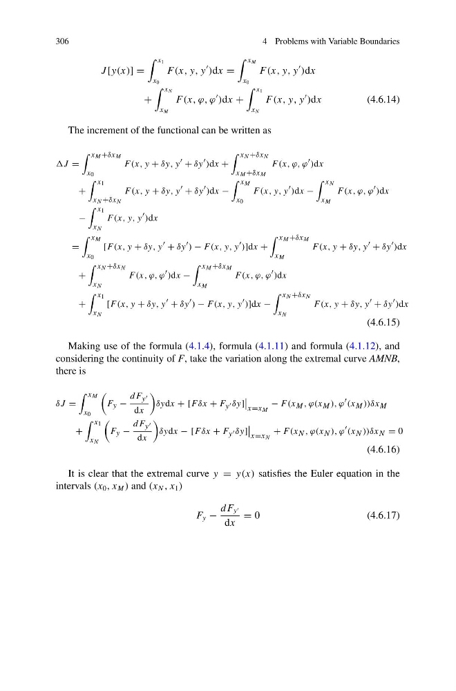
The increment of the functional can be written as
J =
x M +δx M
x 0
F(x, y + δy, y + δy )dx +
x N +δx N
x M +δx M
F(x, ϕ, ϕ )dx
+
x 1
x N +δx N
F(x, y + δy, y + δy )dx −
x M
x 0
F(x, y, y )dx −
x N
x M
F(x, ϕ, ϕ )dx
−
x 1
x N
F(x, y, y )dx
=
x M
x 0
[F(x, y + δy, y + δy ) − F(x, y, y )]dx +
x M +δx M
x M
F(x, y + δy, y + δy )dx
+
x N +δx N
x N
F(x, ϕ, ϕ )dx −
x M +δx M
x M
F(x, ϕ, ϕ )dx
+
x 1
x N
[F(x, y + δy, y + δy ) − F(x, y, y )]dx −
x N +δx N
x N
F(x, y + δy, y + δy )dx
(4.6.15)
Making use of the formula (4.1.4), formula (4.1.11) and formula (4.1.12), and
considering the continuity of F, take the variation along the extremal curve AMNB,
there is
δ J =
x M
x 0
F y −
d F y
dx
δydx + [Fδx + F y δy]
x=x M
− F(x M , ϕ(x M ), ϕ (x M ))δx M
+
x 1
x N
F y −
d F y
dx
δydx − [Fδx + F y δy]
x=x N
+ F(x N , ϕ(x N ), ϕ (x N ))δx N = 0
(4.6.16)
It is clear that the extremal curve y = y(x) satisfies the Euler equation in the
intervals (x 0 , x M ) and (x N , x 1 )
F y −
d F y
dx
= 0
(4.6.17)
4 Problems with Variable Boundaries
J [y(x)] =
x 1
x 0
F(x, y, y
)dx =
x M
x 0
F(x, y, y
)dx
+
x N
x M
F(x, ϕ, ϕ
)dx +
x 1
x N
F(x, y, y
)dx
(4.6.14)
The increment of the functional can be written as
J =
x M +δx M
x 0
F(x, y + δy, y + δy )dx +
x N +δx N
x M +δx M
F(x, ϕ, ϕ )dx
+
x 1
x N +δx N
F(x, y + δy, y + δy )dx −
x M
x 0
F(x, y, y )dx −
x N
x M
F(x, ϕ, ϕ )dx
−
x 1
x N
F(x, y, y )dx
=
x M
x 0
[F(x, y + δy, y + δy ) − F(x, y, y )]dx +
x M +δx M
x M
F(x, y + δy, y + δy )dx
+
x N +δx N
x N
F(x, ϕ, ϕ )dx −
x M +δx M
x M
F(x, ϕ, ϕ )dx
+
x 1
x N
[F(x, y + δy, y + δy ) − F(x, y, y )]dx −
x N +δx N
x N
F(x, y + δy, y + δy )dx
(4.6.15)
Making use of the formula (4.1.4), formula (4.1.11) and formula (4.1.12), and
considering the continuity of F, take the variation along the extremal curve AMNB,
there is
δ J =
x M
x 0
F y −
d F y
dx
δydx + [Fδx + F y δy]
x=x M
− F(x M , ϕ(x M ), ϕ (x M ))δx M
+
x 1
x N
F y −
d F y
dx
δydx − [Fδx + F y δy]
x=x N
+ F(x N , ϕ(x N ), ϕ (x N ))δx N = 0
(4.6.16)
It is clear that the extremal curve y = y(x) satisfies the Euler equation in the
intervals (x 0 , x M ) and (x N , x 1 )
F y −
d F y
dx
= 0
(4.6.17)