

304
4 Problems with Variable Boundaries
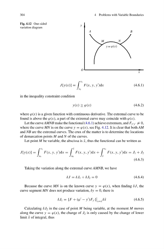
Fig. 4.12 One-sided
variation diagram
O
x
y
A
B
M
N
y = ϕ(x)
J [y(x)] =
x 1
x 0
F(x, y, y
)dx
(4.6.1)
in the inequality constraint condition
y(x) ≥ ϕ(x)
(4.6.2)
where ϕ(x) is a given function with continuous derivative. The extremal curve to be
found is above the ϕ(x), a part of the extremal curve may coincide with ϕ(x).
Let the curve AMNB make the functional (4.6.1) achieve extremum, and F y y = 0,
where the curve MN is on the curve y = ϕ(x), see Fig. 4.12. It is clear that both AM
and NB are the extremal curves. The crux of the matter is to determine the locations
of demarcation points M and N of the curves.
Let point M be variable, the abscissa is ¯
x, thus the functional can be written as
J [y(x)] =
x 1
x 0
F(x, y, y
)dx =
¯
x
x 0
F(x, y, y
)dx +
x 1
¯
x
F(x, y, y
)dx = J 1 + J 2
(4.6.3)
Taking the variation along the extremal curve AMNB, we have
δ J = δ J 1 + δ J 2 = 0
(4.6.4)
Because the curve MN is on the known curve y = ϕ(x), when finding δ J , the
curve segment MN does not produce variation, δy = 0, there is
δ J 1 = [F + (ϕ
− y
)F y ]
x= ¯
x
δ ¯
x
(4.6.5)
Calculating δ J 2 in the case of point M being variable, at the moment M moves
along the curve y = ϕ(x), the change of J 2 is only caused by the change of lower
limit ¯
x of integral, thus
4 Problems with Variable Boundaries
Fig. 4.12 One-sided
variation diagram
O
x
y
A
B
M
N
y = ϕ(x)
J [y(x)] =
x 1
x 0
F(x, y, y
)dx
(4.6.1)
in the inequality constraint condition
y(x) ≥ ϕ(x)
(4.6.2)
where ϕ(x) is a given function with continuous derivative. The extremal curve to be
found is above the ϕ(x), a part of the extremal curve may coincide with ϕ(x).
Let the curve AMNB make the functional (4.6.1) achieve extremum, and F y y = 0,
where the curve MN is on the curve y = ϕ(x), see Fig. 4.12. It is clear that both AM
and NB are the extremal curves. The crux of the matter is to determine the locations
of demarcation points M and N of the curves.
Let point M be variable, the abscissa is ¯
x, thus the functional can be written as
J [y(x)] =
x 1
x 0
F(x, y, y
)dx =
¯
x
x 0
F(x, y, y
)dx +
x 1
¯
x
F(x, y, y
)dx = J 1 + J 2
(4.6.3)
Taking the variation along the extremal curve AMNB, we have
δ J = δ J 1 + δ J 2 = 0
(4.6.4)
Because the curve MN is on the known curve y = ϕ(x), when finding δ J , the
curve segment MN does not produce variation, δy = 0, there is
δ J 1 = [F + (ϕ
− y
)F y ]
x= ¯
x
δ ¯
x
(4.6.5)
Calculating δ J 2 in the case of point M being variable, at the moment M moves
along the curve y = ϕ(x), the change of J 2 is only caused by the change of lower
limit ¯
x of integral, thus