

4.4 Variational Problems of Functionals with Functions of Several Variables
295
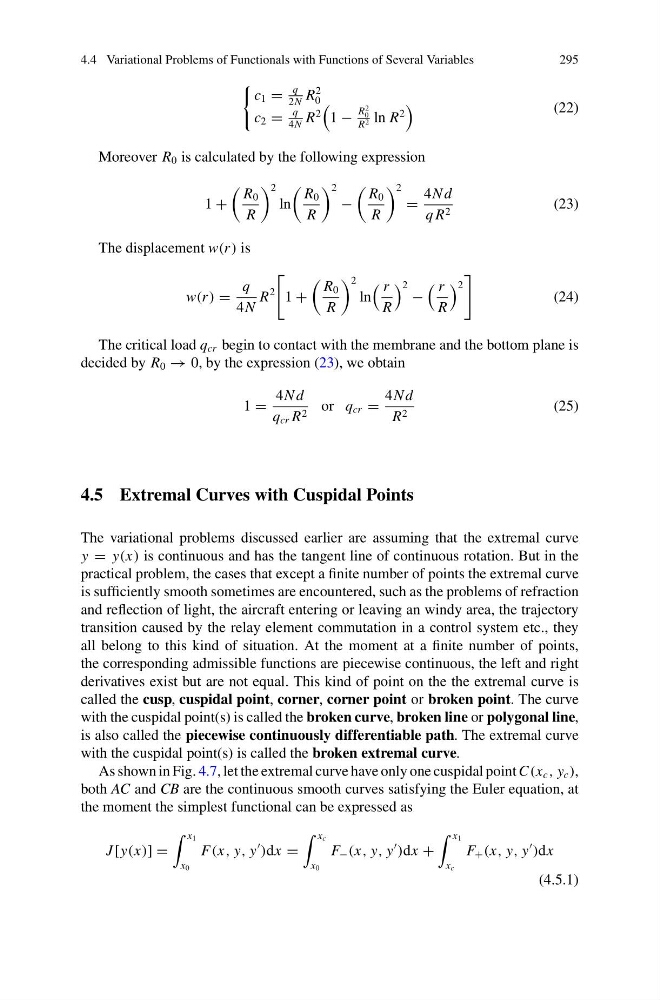
c 1 =
q
2N
R
2
0
c 2 =
q
4N
R
2
1 −
R
2
0
R 2 ln R
2
(22)
Moreover R 0 is calculated by the following expression
1 +
R 0
R
2
ln
R 0
R
2
−
R 0
R
2
=
4N d
q R 2
(23)
The displacement w(r ) is
w(r ) =
q
4N
R
2
1 +
R 0
R
2
ln
r
R
2 −
r
R
2
(24)
The critical load q cr begin to contact with the membrane and the bottom plane is
decided by R 0 → 0, by the expression (23), we obtain
1 =
4N d
q cr R 2 or q cr =
4N d
R 2
(25)
4.5 Extremal Curves with Cuspidal Points
The variational problems discussed earlier are assuming that the extremal curve
y = y(x) is continuous and has the tangent line of continuous rotation. But in the
practical problem, the cases that except a finite number of points the extremal curve
is sufficiently smooth sometimes are encountered, such as the problems of refraction
and reflection of light, the aircraft entering or leaving an windy area, the trajectory
transition caused by the relay element commutation in a control system etc., they
all belong to this kind of situation. At the moment at a finite number of points,
the corresponding admissible functions are piecewise continuous, the left and right
derivatives exist but are not equal. This kind of point on the the extremal curve is
called the cusp, cuspidal point, corner, corner point or broken point. The curve
with the cuspidal point(s) is called the broken curve, broken line or polygonal line,
is also called the piecewise continuously differentiable path. The extremal curve
with the cuspidal point(s) is called the broken extremal curve.
As shown in Fig. 4.7, let the extremal curve have only one cuspidal point C(x c , y c ),
both AC and CB are the continuous smooth curves satisfying the Euler equation, at
the moment the simplest functional can be expressed as
J [y(x)] =
x 1
x 0
F(x, y, y
)dx =
x c
x 0
F − (x, y, y
)dx +
x 1
x c
F + (x, y, y
)dx
(4.5.1)
295
c 1 =
q
2N
R
2
0
c 2 =
q
4N
R
2
1 −
R
2
0
R 2 ln R
2
(22)
Moreover R 0 is calculated by the following expression
1 +
R 0
R
2
ln
R 0
R
2
−
R 0
R
2
=
4N d
q R 2
(23)
The displacement w(r ) is
w(r ) =
q
4N
R
2
1 +
R 0
R
2
ln
r
R
2 −
r
R
2
(24)
The critical load q cr begin to contact with the membrane and the bottom plane is
decided by R 0 → 0, by the expression (23), we obtain
1 =
4N d
q cr R 2 or q cr =
4N d
R 2
(25)
4.5 Extremal Curves with Cuspidal Points
The variational problems discussed earlier are assuming that the extremal curve
y = y(x) is continuous and has the tangent line of continuous rotation. But in the
practical problem, the cases that except a finite number of points the extremal curve
is sufficiently smooth sometimes are encountered, such as the problems of refraction
and reflection of light, the aircraft entering or leaving an windy area, the trajectory
transition caused by the relay element commutation in a control system etc., they
all belong to this kind of situation. At the moment at a finite number of points,
the corresponding admissible functions are piecewise continuous, the left and right
derivatives exist but are not equal. This kind of point on the the extremal curve is
called the cusp, cuspidal point, corner, corner point or broken point. The curve
with the cuspidal point(s) is called the broken curve, broken line or polygonal line,
is also called the piecewise continuously differentiable path. The extremal curve
with the cuspidal point(s) is called the broken extremal curve.
As shown in Fig. 4.7, let the extremal curve have only one cuspidal point C(x c , y c ),
both AC and CB are the continuous smooth curves satisfying the Euler equation, at
the moment the simplest functional can be expressed as
J [y(x)] =
x 1
x 0
F(x, y, y
)dx =
x c
x 0
F − (x, y, y
)dx +
x 1
x c
F + (x, y, y
)dx
(4.5.1)