

4.3 Variational Problems of Functionals with Higher Order Derivatives
275
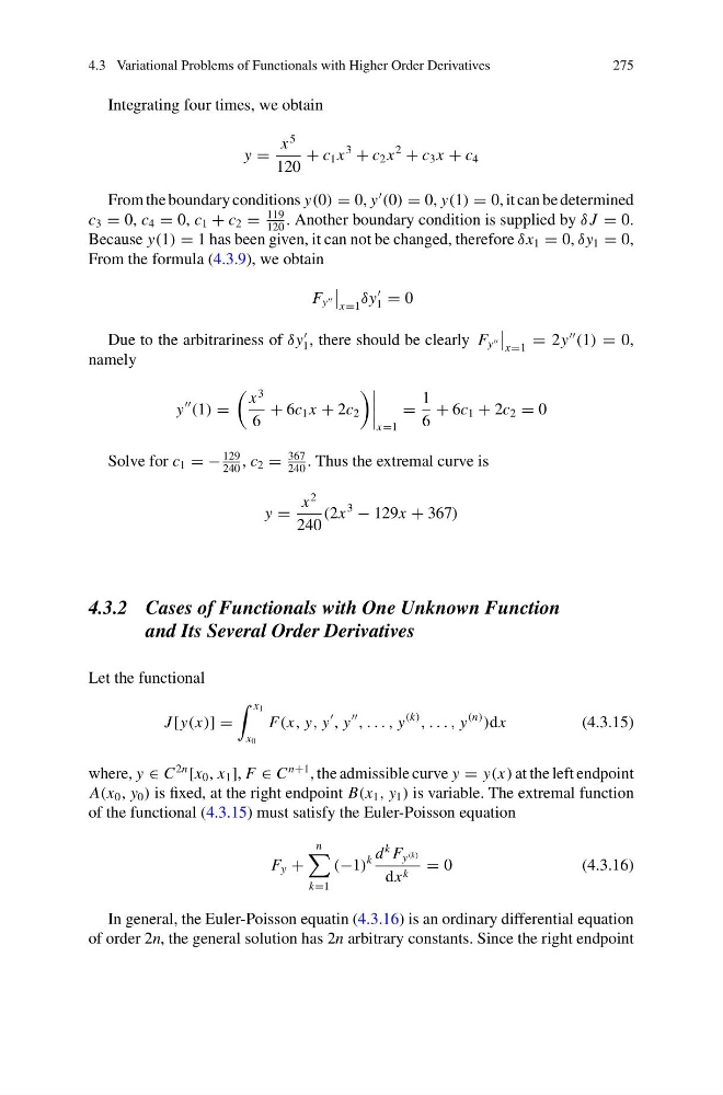
Integrating four times, we obtain
y =
x
5
120
+ c 1 x
3
+ c 2 x
2
+ c 3 x + c 4
From the boundary conditions y(0) = 0, y
(0) = 0, y(1) = 0, it can be determined
c 3 = 0, c 4 = 0, c 1 + c 2 =
119
120
. Another boundary condition is supplied by δ J = 0.
Because y(1) = 1 has been given, it can not be changed, therefore δx 1 = 0, δy 1 = 0,
From the formula (4.3.9), we obtain
F y
x=1
δy
1 = 0
Due to the arbitrariness of δy
1 , there should be clearly F y
x=1
= 2y
(1) = 0,
namely
y
(1) =
x
3
6
+ 6c 1 x + 2c 2
x=1
=
1
6
+ 6c 1 + 2c 2 = 0
Solve for c 1 = −
129
240
, c 2 =
367
240
. Thus the extremal curve is
y =
x
2
240
(2x
3
− 129x + 367)
4.3.2 Cases of Functionals with One Unknown Function
and Its Several Order Derivatives
Let the functional
J [y(x)] =
x 1
x 0
F(x, y, y
, y
, . . . , y
(k)
, . . . , y
(n)
)dx
(4.3.15)
where, y ∈ C
2n
[x 0 , x 1 ], F ∈ C
n+1 , the admissible curve y = y(x) at the left endpoint
A(x 0 , y 0 ) is fixed, at the right endpoint B(x 1 , y 1 ) is variable. The extremal function
of the functional (4.3.15) must satisfy the Euler-Poisson equation
F y +
n
k=1
(−1)
k d
k F y (k)
dx k = 0
(4.3.16)
In general, the Euler-Poisson equatin (4.3.16) is an ordinary differential equation
of order 2n, the general solution has 2n arbitrary constants. Since the right endpoint
275
Integrating four times, we obtain
y =
x
5
120
+ c 1 x
3
+ c 2 x
2
+ c 3 x + c 4
From the boundary conditions y(0) = 0, y
(0) = 0, y(1) = 0, it can be determined
c 3 = 0, c 4 = 0, c 1 + c 2 =
119
120
. Another boundary condition is supplied by δ J = 0.
Because y(1) = 1 has been given, it can not be changed, therefore δx 1 = 0, δy 1 = 0,
From the formula (4.3.9), we obtain
F y
x=1
δy
1 = 0
Due to the arbitrariness of δy
1 , there should be clearly F y
x=1
= 2y
(1) = 0,
namely
y
(1) =
x
3
6
+ 6c 1 x + 2c 2
x=1
=
1
6
+ 6c 1 + 2c 2 = 0
Solve for c 1 = −
129
240
, c 2 =
367
240
. Thus the extremal curve is
y =
x
2
240
(2x
3
− 129x + 367)
4.3.2 Cases of Functionals with One Unknown Function
and Its Several Order Derivatives
Let the functional
J [y(x)] =
x 1
x 0
F(x, y, y
, y
, . . . , y
(k)
, . . . , y
(n)
)dx
(4.3.15)
where, y ∈ C
2n
[x 0 , x 1 ], F ∈ C
n+1 , the admissible curve y = y(x) at the left endpoint
A(x 0 , y 0 ) is fixed, at the right endpoint B(x 1 , y 1 ) is variable. The extremal function
of the functional (4.3.15) must satisfy the Euler-Poisson equation
F y +
n
k=1
(−1)
k d
k F y (k)
dx k = 0
(4.3.16)
In general, the Euler-Poisson equatin (4.3.16) is an ordinary differential equation
of order 2n, the general solution has 2n arbitrary constants. Since the right endpoint