

4.3 Variational Problems of Functionals with Higher Order Derivatives
273
F + (ϕ
− y
)
F y −
d
dx
F y
+ (ψ
− y
)F y
x=x 1
= 0
(4.3.11)
Proof Since y 1 = ϕ(x 1 ), y
1 = ψ(x 1 ), therefore there is
δy 1 = ϕ
(x 1 )δx 1 , δy
1 = ψ
(x 1 )δx 1
(4.3.12)
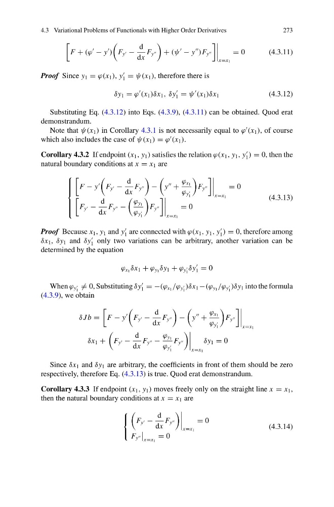
Substituting Eq. (4.3.12) into Eqs. (4.3.9), (4.3.11) can be obtained. Quod erat
demonstrandum.
Note that ψ(x 1 ) in Corollary 4.3.1 is not necessarily equal to ϕ
(x 1 ), of course
which also includes the case of ψ(x 1 ) = ϕ
(x 1 ).
Corollary 4.3.2 If endpoint (x 1 , y 1 ) satisfies the relation ϕ(x 1 , y 1 , y
1 ) = 0, then the
natural boundary conditions at x = x 1 are
⎧
⎪ ⎪ ⎪ ⎨
⎪ ⎪ ⎪ ⎩
F − y
F y −
d
dx
F y
−
y
+
ϕ x 1
ϕ y
1
F y
x=x 1
= 0
F y −
d
dx
F y −
ϕ y 1
ϕ y
1
F y
x=x 1
= 0
(4.3.13)
Proof Because x 1 , y 1 and y
1 are connected with ϕ(x 1 , y 1 , y
1 ) = 0, therefore among
δx 1 , δy 1 and δy
1 only two variations can be arbitrary, another variation can be
determined by the equation
ϕ x 1 δx 1 + ϕ y 1 δy 1 + ϕ y
1
δy
1 = 0
When ϕ y
1
= 0, Substituting δy
1 = −(ϕ x 1 /ϕ y
1
)δx 1 −(ϕ y 1 /ϕ y
1
)δy 1 into the formula
(4.3.9), we obtain
δ J b =
F − y
F y −
d
dx
F y
−
y
+
ϕ x 1
ϕ y
1
F y
x=x 1
δx 1 +
F y −
d
dx
F y −
ϕ y 1
ϕ y
1
F y
x=x 1
δy 1 = 0
Since δx 1 and δy 1 are arbitrary, the coefficients in front of them should be zero
respectively, therefore Eq. (4.3.13) is true. Quod erat demonstrandum.
Corollary 4.3.3 If endpoint (x 1 , y 1 ) moves freely only on the straight line x = x 1 ,
then the natural boundary conditions at x = x 1 are
⎧
⎨
⎩
F y −
d
dx
F y
x=x 1
= 0
F y
x=x 1
= 0
(4.3.14)
273
F + (ϕ
− y
)
F y −
d
dx
F y
+ (ψ
− y
)F y
x=x 1
= 0
(4.3.11)
Proof Since y 1 = ϕ(x 1 ), y
1 = ψ(x 1 ), therefore there is
δy 1 = ϕ
(x 1 )δx 1 , δy
1 = ψ
(x 1 )δx 1
(4.3.12)
Substituting Eq. (4.3.12) into Eqs. (4.3.9), (4.3.11) can be obtained. Quod erat
demonstrandum.
Note that ψ(x 1 ) in Corollary 4.3.1 is not necessarily equal to ϕ
(x 1 ), of course
which also includes the case of ψ(x 1 ) = ϕ
(x 1 ).
Corollary 4.3.2 If endpoint (x 1 , y 1 ) satisfies the relation ϕ(x 1 , y 1 , y
1 ) = 0, then the
natural boundary conditions at x = x 1 are
⎧
⎪ ⎪ ⎪ ⎨
⎪ ⎪ ⎪ ⎩
F − y
F y −
d
dx
F y
−
y
+
ϕ x 1
ϕ y
1
F y
x=x 1
= 0
F y −
d
dx
F y −
ϕ y 1
ϕ y
1
F y
x=x 1
= 0
(4.3.13)
Proof Because x 1 , y 1 and y
1 are connected with ϕ(x 1 , y 1 , y
1 ) = 0, therefore among
δx 1 , δy 1 and δy
1 only two variations can be arbitrary, another variation can be
determined by the equation
ϕ x 1 δx 1 + ϕ y 1 δy 1 + ϕ y
1
δy
1 = 0
When ϕ y
1
= 0, Substituting δy
1 = −(ϕ x 1 /ϕ y
1
)δx 1 −(ϕ y 1 /ϕ y
1
)δy 1 into the formula
(4.3.9), we obtain
δ J b =
F − y
F y −
d
dx
F y
−
y
+
ϕ x 1
ϕ y
1
F y
x=x 1
δx 1 +
F y −
d
dx
F y −
ϕ y 1
ϕ y
1
F y
x=x 1
δy 1 = 0
Since δx 1 and δy 1 are arbitrary, the coefficients in front of them should be zero
respectively, therefore Eq. (4.3.13) is true. Quod erat demonstrandum.
Corollary 4.3.3 If endpoint (x 1 , y 1 ) moves freely only on the straight line x = x 1 ,
then the natural boundary conditions at x = x 1 are
⎧
⎨
⎩
F y −
d
dx
F y
x=x 1
= 0
F y
x=x 1
= 0
(4.3.14)