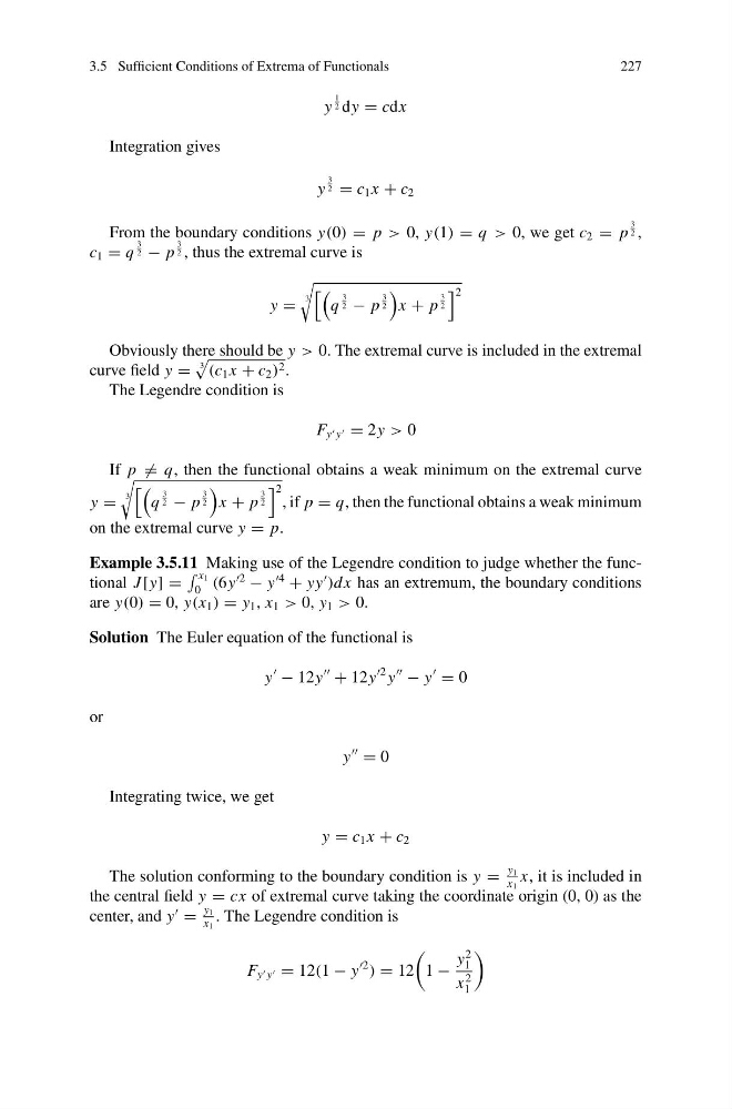
3.5 Sufficient Conditions of Extrema of Functionals
227
y
1
2 dy = cdx
Integration gives
y
3
2 = c 1 x + c 2
From the boundary conditions y(0) = p > 0, y(1) = q > 0, we get c 2 = p
3
2 ,
c 1 = q
3
2 − p
3
2 , thus the extremal curve is
y =
3
q
3
2 − p
3
2
x + p
3
2
2
Obviously there should be y > 0. The extremal curve is included in the extremal
curve field y =
3
(c 1 x + c 2 ) 2 .
The Legendre condition is
F y y = 2y > 0
If p = q, then the functional obtains a weak minimum on the extremal curve
y =
3
q
3
2 − p
3
2
x + p
3
2
2
, if p = q, then the functional obtains a weak minimum
on the extremal curve y = p.
Example 3.5.11 Making use of the Legendre condition to judge whether the functional J [y] =
x 1
0 (6y
2
− y
4
+ yy
)dx has an extremum, the boundary conditions
are y(0) = 0, y(x 1 ) = y 1 , x 1 > 0, y 1 > 0.
Solution The Euler equation of the functional is
y
− 12y
+ 12y
2 y
− y
= 0
or
y
= 0
Integrating twice, we get
y = c 1 x + c 2
The solution conforming to the boundary condition is y =
y 1
x 1
x, it is included in
the central field y = cx of extremal curve taking the coordinate origin (0, 0) as the
center, and y
=
y 1
x 1
. The Legendre condition is
F y y = 12(1 − y
2
) = 12
1 −
y
2
1
x
2
1