

3.3 The Weierstrass Functions and Weierstrass Conditions
213
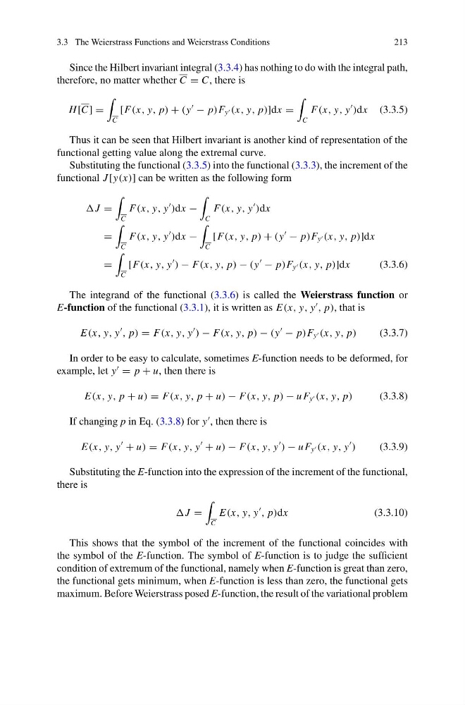
Since the Hilbert invariant integral (3.3.4) has nothing to do with the integral path,
therefore, no matter whether C = C, there is
H [C] =
C
[F(x, y, p) + (y
− p)F y (x, y, p)]dx =
C
F(x, y, y
)dx (3.3.5)
Thus it can be seen that Hilbert invariant is another kind of representation of the
functional getting value along the extremal curve.
Substituting the functional (3.3.5) into the functional (3.3.3), the increment of the
functional J [y(x)] can be written as the following form
J =
C
F(x, y, y
)dx −
C
F(x, y, y
)dx
=
C
F(x, y, y
)dx −
C
[F(x, y, p) + (y
− p)F y (x, y, p)]dx
=
C
[F(x, y, y
) − F(x, y, p) − (y
− p)F y (x, y, p)]dx
(3.3.6)
The integrand of the functional (3.3.6) is called the Weierstrass function or
E-function of the functional (3.3.1), it is written as E(x, y, y
, p), that is
E(x, y, y
, p) = F(x, y, y
) − F(x, y, p) − (y
− p)F y (x, y, p)
(3.3.7)
In order to be easy to calculate, sometimes E-function needs to be deformed, for
example, let y
= p + u, then there is
E(x, y, p + u) = F(x, y, p + u) − F(x, y, p) − u F y (x, y, p)
(3.3.8)
If changing p in Eq. (3.3.8) for y
, then there is
E(x, y, y
+ u) = F(x, y, y
+ u) − F(x, y, y
) − u F y (x, y, y
)
(3.3.9)
Substituting the E-function into the expression of the increment of the functional,
there is
J =
C
E(x, y, y
, p)dx
(3.3.10)
This shows that the symbol of the increment of the functional coincides with
the symbol of the E-function. The symbol of E-function is to judge the sufficient
condition of extremum of the functional, namely when E-function is great than zero,
the functional gets minimum, when E-function is less than zero, the functional gets
maximum. Before Weierstrass posed E-function, the result of the variational problem
213
Since the Hilbert invariant integral (3.3.4) has nothing to do with the integral path,
therefore, no matter whether C = C, there is
H [C] =
C
[F(x, y, p) + (y
− p)F y (x, y, p)]dx =
C
F(x, y, y
)dx (3.3.5)
Thus it can be seen that Hilbert invariant is another kind of representation of the
functional getting value along the extremal curve.
Substituting the functional (3.3.5) into the functional (3.3.3), the increment of the
functional J [y(x)] can be written as the following form
J =
C
F(x, y, y
)dx −
C
F(x, y, y
)dx
=
C
F(x, y, y
)dx −
C
[F(x, y, p) + (y
− p)F y (x, y, p)]dx
=
C
[F(x, y, y
) − F(x, y, p) − (y
− p)F y (x, y, p)]dx
(3.3.6)
The integrand of the functional (3.3.6) is called the Weierstrass function or
E-function of the functional (3.3.1), it is written as E(x, y, y
, p), that is
E(x, y, y
, p) = F(x, y, y
) − F(x, y, p) − (y
− p)F y (x, y, p)
(3.3.7)
In order to be easy to calculate, sometimes E-function needs to be deformed, for
example, let y
= p + u, then there is
E(x, y, p + u) = F(x, y, p + u) − F(x, y, p) − u F y (x, y, p)
(3.3.8)
If changing p in Eq. (3.3.8) for y
, then there is
E(x, y, y
+ u) = F(x, y, y
+ u) − F(x, y, y
) − u F y (x, y, y
)
(3.3.9)
Substituting the E-function into the expression of the increment of the functional,
there is
J =
C
E(x, y, y
, p)dx
(3.3.10)
This shows that the symbol of the increment of the functional coincides with
the symbol of the E-function. The symbol of E-function is to judge the sufficient
condition of extremum of the functional, namely when E-function is great than zero,
the functional gets minimum, when E-function is less than zero, the functional gets
maximum. Before Weierstrass posed E-function, the result of the variational problem