

3.2 The Jacobi Conditions and Jacobi Equation
209
then there is
F y = F y (x, y(x, c 1 , c 2 ), y
(x, c 1 , c 2 ))
(3.2.18)
F y = F y (x, y(x, c 1 , c 2 ), y
(x, c 1 , c 2 ))
(3.2.19)
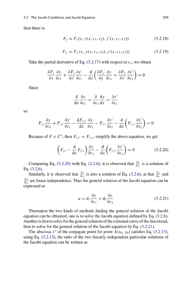
Take the partial derivative of Eq. (3.2.17) with respect to c 1 , we obtain
∂ F y
∂ y
∂ y
∂c 1
+
∂ F y
∂ y
∂ y
∂c 1
−
d
dx
∂ F y
∂ y
∂ y
∂c 1
+
∂ F y
∂ y
∂ y
∂c 1
= 0
Since
d
dx
∂ y
∂c 1
=
∂
∂c 1
dy
dx
=
∂ y
∂c 1
so
F yy
∂ y
∂c 1
+ F yy
∂ y
∂c 1
−
dF y y
dx
∂ y
∂c 1
− F y y
∂ y
∂c 1
−
d
dx
F y y
∂ y
∂c 1
= 0
Because of F ∈ C
2 , then F yy = F y y , simplify the above equation, we get
F yy −
d
dx
F y y
∂ y
∂c 1
−
d
dx
F y y
∂ y
∂c 1
= 0
(3.2.20)
Comparing Eq. (3.2.20) with Eq. (3.2.6), it is observed that
∂ y
∂c 1
is a solution of
Eq. (3.2.6).
Similarly, it is observed that
∂ y
∂c 2
is also a solution of Eq. (3.2.6), at that
∂ y
∂c 1
and
∂ y
∂c 2
are linear independence. Thus the general solution of the Jacobi equation can be
expressed as
u = d 1
∂ y
∂c 1
+ d 2
∂ y
∂c 2
(3.2.21)
Thereupon the two kinds of methods finding the general solution of the Jacobi
equation can be obtained, one is to solve the Jacobi equation defined by Eq. (3.2.6),
Another is first to solve for the general solution of the extremal curve of the functional,
then to solve for the general solution of the Jacobi equation by Eq. (3.2.21).
The abscissa x
∗ of the conjugate point for point A(x 0 , y 0 ) satisfies Eq. (3.2.13),
using Eq. (3.2.13), the ratio of the two linearly independent particular solutions of
the Jacobi equation can be written as
209
then there is
F y = F y (x, y(x, c 1 , c 2 ), y
(x, c 1 , c 2 ))
(3.2.18)
F y = F y (x, y(x, c 1 , c 2 ), y
(x, c 1 , c 2 ))
(3.2.19)
Take the partial derivative of Eq. (3.2.17) with respect to c 1 , we obtain
∂ F y
∂ y
∂ y
∂c 1
+
∂ F y
∂ y
∂ y
∂c 1
−
d
dx
∂ F y
∂ y
∂ y
∂c 1
+
∂ F y
∂ y
∂ y
∂c 1
= 0
Since
d
dx
∂ y
∂c 1
=
∂
∂c 1
dy
dx
=
∂ y
∂c 1
so
F yy
∂ y
∂c 1
+ F yy
∂ y
∂c 1
−
dF y y
dx
∂ y
∂c 1
− F y y
∂ y
∂c 1
−
d
dx
F y y
∂ y
∂c 1
= 0
Because of F ∈ C
2 , then F yy = F y y , simplify the above equation, we get
F yy −
d
dx
F y y
∂ y
∂c 1
−
d
dx
F y y
∂ y
∂c 1
= 0
(3.2.20)
Comparing Eq. (3.2.20) with Eq. (3.2.6), it is observed that
∂ y
∂c 1
is a solution of
Eq. (3.2.6).
Similarly, it is observed that
∂ y
∂c 2
is also a solution of Eq. (3.2.6), at that
∂ y
∂c 1
and
∂ y
∂c 2
are linear independence. Thus the general solution of the Jacobi equation can be
expressed as
u = d 1
∂ y
∂c 1
+ d 2
∂ y
∂c 2
(3.2.21)
Thereupon the two kinds of methods finding the general solution of the Jacobi
equation can be obtained, one is to solve the Jacobi equation defined by Eq. (3.2.6),
Another is first to solve for the general solution of the extremal curve of the functional,
then to solve for the general solution of the Jacobi equation by Eq. (3.2.21).
The abscissa x
∗ of the conjugate point for point A(x 0 , y 0 ) satisfies Eq. (3.2.13),
using Eq. (3.2.13), the ratio of the two linearly independent particular solutions of
the Jacobi equation can be written as