

4
1 Preliminaries
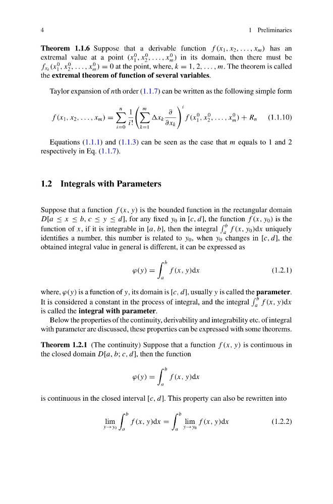
Theorem 1.1.6 Suppose that a derivable function f (x 1 , x 2 , . . . , x m ) has an
extremal value at a point (x
0
1 , x
0
2 , . . . , x
0
m ) in its domain, then there must be
f x k (x
0
1 , x
0
2 , . . . , x
0
m ) = 0 at the point, where, k = 1, 2, . . . , m. The theorem is called
the extremal theorem of function of several variables.
Taylor expansion of nth order (1.1.7) can be written as the following simple form
f (x 1 , x 2 , . . . , x m ) =
n
i=0
1
i!
m
k=1
x k
∂
∂ x k
i
f (x
0
1 , x
0
2 , . . . , x
0
m ) + R n (1.1.10)
Equations (1.1.1) and (1.1.3) can be seen as the case that m equals to 1 and 2
respectively in Eq. (1.1.7).
1.2 Integrals with Parameters
Suppose that a function f (x, y) is the bounded function in the rectangular domain
D[a ≤ x ≤ b, c ≤ y ≤ d], for any fixed y 0 in [c, d], the function f (x, y 0 ) is the
function of x, if it is integrable in [a, b], then the integral
b
a f (x, y 0 )dx uniquely
identifies a number, this number is related to y 0 , when y 0 changes in [c, d], the
obtained integral value in general is different, it can be expressed as
ϕ(y) =
b
a
f (x, y)dx
(1.2.1)
where, ϕ(y) is a function of y, its domain is [c, d], usually y is called the parameter.
It is considered a constant in the process of integral, and the integral
b
a f (x, y)dx
is called the integral with parameter.
Below the properties of the continuity, derivability and integrability etc. of integral
with parameter are discussed, these properties can be expressed with some theorems.
Theorem 1.2.1 (The continuity) Suppose that a function f (x, y) is continuous in
the closed domain D[a, b; c, d], then the function
ϕ(y) =
b
a
f (x, y)dx
is continuous in the closed interval [c, d]. This property can also be rewritten into
lim
y→y 0
b
a
f (x, y)dx =
b
a
lim
y→y 0
f (x, y)dx
(1.2.2)
1 Preliminaries
Theorem 1.1.6 Suppose that a derivable function f (x 1 , x 2 , . . . , x m ) has an
extremal value at a point (x
0
1 , x
0
2 , . . . , x
0
m ) in its domain, then there must be
f x k (x
0
1 , x
0
2 , . . . , x
0
m ) = 0 at the point, where, k = 1, 2, . . . , m. The theorem is called
the extremal theorem of function of several variables.
Taylor expansion of nth order (1.1.7) can be written as the following simple form
f (x 1 , x 2 , . . . , x m ) =
n
i=0
1
i!
m
k=1
x k
∂
∂ x k
i
f (x
0
1 , x
0
2 , . . . , x
0
m ) + R n (1.1.10)
Equations (1.1.1) and (1.1.3) can be seen as the case that m equals to 1 and 2
respectively in Eq. (1.1.7).
1.2 Integrals with Parameters
Suppose that a function f (x, y) is the bounded function in the rectangular domain
D[a ≤ x ≤ b, c ≤ y ≤ d], for any fixed y 0 in [c, d], the function f (x, y 0 ) is the
function of x, if it is integrable in [a, b], then the integral
b
a f (x, y 0 )dx uniquely
identifies a number, this number is related to y 0 , when y 0 changes in [c, d], the
obtained integral value in general is different, it can be expressed as
ϕ(y) =
b
a
f (x, y)dx
(1.2.1)
where, ϕ(y) is a function of y, its domain is [c, d], usually y is called the parameter.
It is considered a constant in the process of integral, and the integral
b
a f (x, y)dx
is called the integral with parameter.
Below the properties of the continuity, derivability and integrability etc. of integral
with parameter are discussed, these properties can be expressed with some theorems.
Theorem 1.2.1 (The continuity) Suppose that a function f (x, y) is continuous in
the closed domain D[a, b; c, d], then the function
ϕ(y) =
b
a
f (x, y)dx
is continuous in the closed interval [c, d]. This property can also be rewritten into
lim
y→y 0
b
a
f (x, y)dx =
b
a
lim
y→y 0
f (x, y)dx
(1.2.2)