

184
2 Variational Problems with Fixed Boundaries
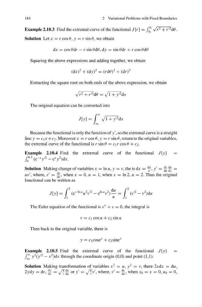
Example 2.10.3 Find the extremal curve of the functional J [r ] =
θ 1
θ 0
√
r 2 + r 2 dθ.
Solution Let x = r cos θ , y = r sin θ , we obtain
dx = cos θ dr − r sin θ dθ, dy = sin θ dr + r cos θ dθ
Squaring the above expressions and adding together, we obtain
(dx)
2
+ (dy)
2
= (r dθ)
2
+ (dr )
2
Extracting the square root on both ends of the above expression, we obtain
r 2 + r 2 dθ =
1 + y 2 dx
The original equation can be converted into
J [y] =
x 1
x 0
1 + y 2 dx
Because the functional is only the function of y
, so the extremal curve is a straight
line y = c 1 x +c 2 . Moreover x = r cos θ , y = r sin θ , return to the original variables,
the extremal curve of the functional is r sin θ = c 1 r cos θ + c 2 .
Example 2.10.4 Find the extremal curve of the functional J [y] =
ln 2
0
(e
−x y
2
− e
x y
2
)dx.
Solution Making change of variables x = ln u, y = v, the is dx =
du
u
, y
=
dv
du
du
dx
=
uv
, where, v
=
dv
du
, when x = 0, u = 1, when x = ln 2, u = 2. Thus the original
functional can be written as
J [y] =
2
1
(e
− ln u u
2 v
2
− e
ln u v
2
)
du
u
=
2
1
(v
2
− v
2
)du
The Euler equation of the functional is v
+ v = 0, the integral is
v = c 1 cos u + c 2 sin u
Then back to the original variable, there is
y = c 1 cose
x
+ c 2 sine
x
Example 2.10.5 Find the extremal curve of the functional J [y] =
x 1
x 0
y
2
(y
2
− x
2
)dx through the coordinate origin (0,0) and point (1,1).
Solution Making transformation of variables x
2
= u, y
2
= v, there 2xdx = du,
2ydy = dv,
dy
dx
=
u
v
dv
du
or y
=
u
v
v
, where, v
=
dv
du
, when x 0 = x = 0, u 0 = 0,
2 Variational Problems with Fixed Boundaries
Example 2.10.3 Find the extremal curve of the functional J [r ] =
θ 1
θ 0
√
r 2 + r 2 dθ.
Solution Let x = r cos θ , y = r sin θ , we obtain
dx = cos θ dr − r sin θ dθ, dy = sin θ dr + r cos θ dθ
Squaring the above expressions and adding together, we obtain
(dx)
2
+ (dy)
2
= (r dθ)
2
+ (dr )
2
Extracting the square root on both ends of the above expression, we obtain
r 2 + r 2 dθ =
1 + y 2 dx
The original equation can be converted into
J [y] =
x 1
x 0
1 + y 2 dx
Because the functional is only the function of y
, so the extremal curve is a straight
line y = c 1 x +c 2 . Moreover x = r cos θ , y = r sin θ , return to the original variables,
the extremal curve of the functional is r sin θ = c 1 r cos θ + c 2 .
Example 2.10.4 Find the extremal curve of the functional J [y] =
ln 2
0
(e
−x y
2
− e
x y
2
)dx.
Solution Making change of variables x = ln u, y = v, the is dx =
du
u
, y
=
dv
du
du
dx
=
uv
, where, v
=
dv
du
, when x = 0, u = 1, when x = ln 2, u = 2. Thus the original
functional can be written as
J [y] =
2
1
(e
− ln u u
2 v
2
− e
ln u v
2
)
du
u
=
2
1
(v
2
− v
2
)du
The Euler equation of the functional is v
+ v = 0, the integral is
v = c 1 cos u + c 2 sin u
Then back to the original variable, there is
y = c 1 cose
x
+ c 2 sine
x
Example 2.10.5 Find the extremal curve of the functional J [y] =
x 1
x 0
y
2
(y
2
− x
2
)dx through the coordinate origin (0,0) and point (1,1).
Solution Making transformation of variables x
2
= u, y
2
= v, there 2xdx = du,
2ydy = dv,
dy
dx
=
u
v
dv
du
or y
=
u
v
v
, where, v
=
dv
du
, when x 0 = x = 0, u 0 = 0,