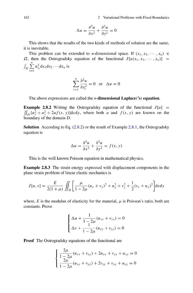
162
2 Variational Problems with Fixed Boundaries
u =
∂
2 u
∂ x 2 +
∂
2 u
∂ y 2 = 0
This shows that the results of the two kinds of methods of solution are the same,
it is inevitable.
This problem can be extended to n-dimensional space. If (x 1 , x 2 , · · · , x n ) ∈
Ω, then the Ostrogradsky equation of the functional J [u(x 1 , x 2 , · · · , x n )] =
Ω
n
i=1
u
2
x i
dx 1 dx 2 · · · dx n is
n
i=1
∂
2 u
∂ x
2
i
= 0 or u = 0
The above expressions are called the n-dimensional Laplace(’s) equation.
Example 2.8.2 Writing the Ostrogradsky equation of the functional J [u] =
˜
D [u
2
x + u
2
y + 2u f (x, y)]dxdy, where both u and f (x, y) are known on the
boundary of the domain D.
Solution According to Eq. (2.8.2) or the result of Example 2.8.1, the Ostrogradsky
equation is
u =
∂
2 u
∂ x 2 +
∂
2 u
∂ y 2 = f (x, y)
This is the well known Poisson equation in mathematical physics.
Example 2.8.3 The strain energy expressed with displacement components in the
plane strain problem of linear elastic mechanics is
J [u, v] =
E
2(1 + μ)
¨
D
μ
1 − 2μ
(u x + v y )
2
+ u
2
x + v
2
y +
1
2
(v x + u y )
2
dxdy
where, E is the modulus of elasticity for the material, μ is Poisson’s ratio, both are
constants. Prove
⎧
⎪ ⎨
⎪ ⎩
u +
1
1 − 2μ
(u xx + v xy ) = 0
v +
1
1 − 2μ
(u xy + v yy ) = 0
Proof The Ostrogradsky equations of the functional are
⎧
⎪ ⎨
⎪ ⎩
2μ
1 − 2μ
(u xx + v xy ) + 2u xx + v xy + u yy = 0
2μ
1 − 2μ
(u xy + v yy ) + 2v yy + v xx + u xy = 0