

136
2 Variational Problems with Fixed Boundaries
O
x
y
a
θ
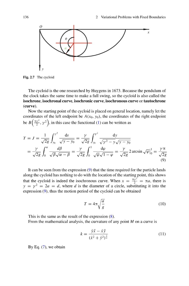
Fig. 2.7 The cycloid
The cycloid is the one researched by Huygens in 1673. Because the pendulum of
the clock takes the same time to make a full swing, so the cycloid is also called the
isochrone, isochronal curve, isochronic curve, isochronous curve or tautochrone
(curve).
Now the starting point of the cycloid is placed on general location, namely let the
coordinates of the left endpoint be A(x 0 , y 0 ), the coordinates of the right endpoint
be B
πγ
2
2
, γ
2
, in this case the functional (1) can be written as
T = J =
1
√
2g
γ
2
y 0
ds
√ y − y 0
=
γ
√
2g
γ
2
y 0
dy
γ 2 − y
√ y − y 0
=
γ
√
2g
α
0
dβ
√ β
√
α − β
=
γ
√
2g
1
0
dϕ
√ ϕ
√
1 − ϕ
=
γ
√
2g
2 arcsin
√
ϕ
1
0
=
γ π
√
2g
(9)
It can be seen from the expression (9) that the time required for the particle lands
along the cycloid has nothing to do with the location of the starting point, this shows
that the cycloid is indeed the isochronous curve. When x =
πγ
2
2
= πa, there is
y = γ
2
= 2a = d, where d is the diameter of a circle, substituting it into the
expression (9), thus the motion period of the cycloid can be obtained
T = 4π
a
g
(10)
This is the same as the result of the expression (8).
From the mathematical analysis, the curvature of any point M on a curve is
k =
˙
y ¨
x − ˙
x ¨
y
( ˙
x 2 + ˙
y 2 )
3
2
(11)
By Eq. (7), we obtain
2 Variational Problems with Fixed Boundaries
O
x
y
a
θ
Fig. 2.7 The cycloid
The cycloid is the one researched by Huygens in 1673. Because the pendulum of
the clock takes the same time to make a full swing, so the cycloid is also called the
isochrone, isochronal curve, isochronic curve, isochronous curve or tautochrone
(curve).
Now the starting point of the cycloid is placed on general location, namely let the
coordinates of the left endpoint be A(x 0 , y 0 ), the coordinates of the right endpoint
be B
πγ
2
2
, γ
2
, in this case the functional (1) can be written as
T = J =
1
√
2g
γ
2
y 0
ds
√ y − y 0
=
γ
√
2g
γ
2
y 0
dy
γ 2 − y
√ y − y 0
=
γ
√
2g
α
0
dβ
√ β
√
α − β
=
γ
√
2g
1
0
dϕ
√ ϕ
√
1 − ϕ
=
γ
√
2g
2 arcsin
√
ϕ
1
0
=
γ π
√
2g
(9)
It can be seen from the expression (9) that the time required for the particle lands
along the cycloid has nothing to do with the location of the starting point, this shows
that the cycloid is indeed the isochronous curve. When x =
πγ
2
2
= πa, there is
y = γ
2
= 2a = d, where d is the diameter of a circle, substituting it into the
expression (9), thus the motion period of the cycloid can be obtained
T = 4π
a
g
(10)
This is the same as the result of the expression (8).
From the mathematical analysis, the curvature of any point M on a curve is
k =
˙
y ¨
x − ˙
x ¨
y
( ˙
x 2 + ˙
y 2 )
3
2
(11)
By Eq. (7), we obtain