

110
2 Variational Problems with Fixed Boundaries
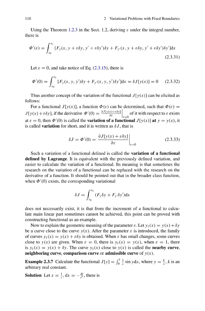
Using the Theorem 1.2.3 in the Sect. 1.2, deriving ε under the integral number,
there is
Φ
(ε) =
x 1
x 0
[F y (x, y + εδy, y
+ εδy
)δy + F y (x, y + εδy, y
+ εδy
)δy
]dx
(2.3.31)
Let ε = 0, and take notice of Eq. (2.3.15), there is
Φ
(0) =
x 1
x 0
[F y (x, y, y
)δy + F y (x, y, y
)δy
]dx = δ J [y(x)] = 0 (2.3.32)
Thus another concept of the variation of the functional J [y(x)] can be elicited as
follows:
For a functional J [y(x)], a function Φ(ε) can be determined, such that Φ(ε) =
J [y(x) + εδy], if the derivative Φ
(0) =
∂ J [y(x)+εδy]
∂ε
ε=0
of it with respect to ε exists
at ε = 0, then Φ
(0) is called the variation of a functional J [y(x)] at y = y(x), it
is called variation for short, and it is written as δ J , that is
δ J = Φ
(0) =
∂ J [y(x) + εδy]
∂ε
ε=0
(2.3.33)
Such a variation of a functional defined is called the variation of a functional
defined by Lagrange. It is equivalent with the previously defined variation, and
easier to calculate the variation of a functional. Its meaning is that sometimes the
research on the variation of a functional can be replaced with the research on the
derivative of a function. It should be pointed out that in the broader class function,
when Φ
(0) exists, the corresponding variational
δ J =
x 1
x 0
(F y δy + F y δy
)dx
does not necessarily exist, it is that from the increment of a functional to calculate main linear part sometimes cannot be achieved, this point can be proved with
constructing functional as an example.
Now to explain the geometric meaning of the parameter ε. Let y 1 (x) = y(x) + δy
be a curve close to the curve y(x). After the parameter ε is introduced, the family
of curves y 1 (x) = y(x) + εδy is obtained. When ε has small changes, some curves
close to y(x) are given. When ε = 0, there is y 1 (x) = y(x), when ε = 1, there
is y 1 (x) = y(x) + δy. The curve y 1 (x) close to y(x) is called the nearby curve,
neighboring curve, comparison curve or admissible curve of y(x).
Example 2.3.7 Calculate the functional J [y] =
1
0
1
x
sin ydx, where y =
k
x
, k is an
arbitrary real constant.
Solution Let x =
1
t
, dx = −
dt
t 2 , there is
2 Variational Problems with Fixed Boundaries
Using the Theorem 1.2.3 in the Sect. 1.2, deriving ε under the integral number,
there is
Φ
(ε) =
x 1
x 0
[F y (x, y + εδy, y
+ εδy
)δy + F y (x, y + εδy, y
+ εδy
)δy
]dx
(2.3.31)
Let ε = 0, and take notice of Eq. (2.3.15), there is
Φ
(0) =
x 1
x 0
[F y (x, y, y
)δy + F y (x, y, y
)δy
]dx = δ J [y(x)] = 0 (2.3.32)
Thus another concept of the variation of the functional J [y(x)] can be elicited as
follows:
For a functional J [y(x)], a function Φ(ε) can be determined, such that Φ(ε) =
J [y(x) + εδy], if the derivative Φ
(0) =
∂ J [y(x)+εδy]
∂ε
ε=0
of it with respect to ε exists
at ε = 0, then Φ
(0) is called the variation of a functional J [y(x)] at y = y(x), it
is called variation for short, and it is written as δ J , that is
δ J = Φ
(0) =
∂ J [y(x) + εδy]
∂ε
ε=0
(2.3.33)
Such a variation of a functional defined is called the variation of a functional
defined by Lagrange. It is equivalent with the previously defined variation, and
easier to calculate the variation of a functional. Its meaning is that sometimes the
research on the variation of a functional can be replaced with the research on the
derivative of a function. It should be pointed out that in the broader class function,
when Φ
(0) exists, the corresponding variational
δ J =
x 1
x 0
(F y δy + F y δy
)dx
does not necessarily exist, it is that from the increment of a functional to calculate main linear part sometimes cannot be achieved, this point can be proved with
constructing functional as an example.
Now to explain the geometric meaning of the parameter ε. Let y 1 (x) = y(x) + δy
be a curve close to the curve y(x). After the parameter ε is introduced, the family
of curves y 1 (x) = y(x) + εδy is obtained. When ε has small changes, some curves
close to y(x) are given. When ε = 0, there is y 1 (x) = y(x), when ε = 1, there
is y 1 (x) = y(x) + δy. The curve y 1 (x) close to y(x) is called the nearby curve,
neighboring curve, comparison curve or admissible curve of y(x).
Example 2.3.7 Calculate the functional J [y] =
1
0
1
x
sin ydx, where y =
k
x
, k is an
arbitrary real constant.
Solution Let x =
1
t
, dx = −
dt
t 2 , there is