

5.4 Geodesics as Self-parallel Curves
67
5.4 Geodesics as Self-parallel Curves
We now know how to displace a vector to a nearby point so that it remains parallel to
itself in the general sense defined in the preceding two sections. We may use this to
define and study the idea of a generalized straight line or geodesic. Our definition of
a geodesic stems naturally from classical Euclidean geometry and intuition. Suppose
we have a curve C specified by giving the coordinates as functions of some scalar
parameter p which labels points on C,
Curve C: x
μ
= x
μ
( p).
(5.22)
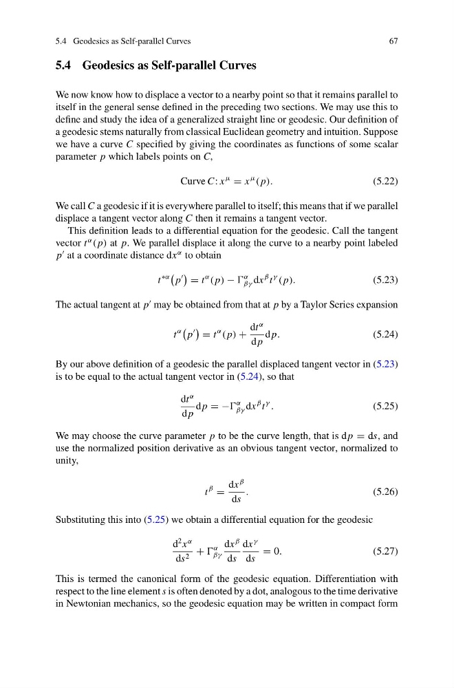
We call C a geodesic if it is everywhere parallel to itself; this means that if we parallel
displace a tangent vector along C then it remains a tangent vector.
This definition leads to a differential equation for the geodesic. Call the tangent
vector t
α
( p) at p. We parallel displace it along the curve to a nearby point labeled
p
at a coordinate distance dx
α to obtain
t
∗α
p
= t
α
( p) −
α
βγ dx
β t
γ
( p).
(5.23)
The actual tangent at p
may be obtained from that at p by a Taylor Series expansion
t
α
p
= t
α
( p) +
dt
α
d p
d p.
(5.24)
By our above definition of a geodesic the parallel displaced tangent vector in (5.23)
is to be equal to the actual tangent vector in (5.24), so that
dt
α
d p
d p = −
α
βγ dx
β t
γ
.
(5.25)
We may choose the curve parameter p to be the curve length, that is d p = ds, and
use the normalized position derivative as an obvious tangent vector, normalized to
unity,
t
β
=
dx
β
ds
.
(5.26)
Substituting this into (5.25) we obtain a differential equation for the geodesic
d
2 x
α
ds 2 +
α
βγ
dx
β
ds
dx
γ
ds
= 0.
(5.27)
This is termed the canonical form of the geodesic equation. Differentiation with
respect to the line element s is often denoted by a dot, analogous to the time derivative
in Newtonian mechanics, so the geodesic equation may be written in compact form
67
5.4 Geodesics as Self-parallel Curves
We now know how to displace a vector to a nearby point so that it remains parallel to
itself in the general sense defined in the preceding two sections. We may use this to
define and study the idea of a generalized straight line or geodesic. Our definition of
a geodesic stems naturally from classical Euclidean geometry and intuition. Suppose
we have a curve C specified by giving the coordinates as functions of some scalar
parameter p which labels points on C,
Curve C: x
μ
= x
μ
( p).
(5.22)
We call C a geodesic if it is everywhere parallel to itself; this means that if we parallel
displace a tangent vector along C then it remains a tangent vector.
This definition leads to a differential equation for the geodesic. Call the tangent
vector t
α
( p) at p. We parallel displace it along the curve to a nearby point labeled
p
at a coordinate distance dx
α to obtain
t
∗α
p
= t
α
( p) −
α
βγ dx
β t
γ
( p).
(5.23)
The actual tangent at p
may be obtained from that at p by a Taylor Series expansion
t
α
p
= t
α
( p) +
dt
α
d p
d p.
(5.24)
By our above definition of a geodesic the parallel displaced tangent vector in (5.23)
is to be equal to the actual tangent vector in (5.24), so that
dt
α
d p
d p = −
α
βγ dx
β t
γ
.
(5.25)
We may choose the curve parameter p to be the curve length, that is d p = ds, and
use the normalized position derivative as an obvious tangent vector, normalized to
unity,
t
β
=
dx
β
ds
.
(5.26)
Substituting this into (5.25) we obtain a differential equation for the geodesic
d
2 x
α
ds 2 +
α
βγ
dx
β
ds
dx
γ
ds
= 0.
(5.27)
This is termed the canonical form of the geodesic equation. Differentiation with
respect to the line element s is often denoted by a dot, analogous to the time derivative
in Newtonian mechanics, so the geodesic equation may be written in compact form