

20
3 The Motion of Particles
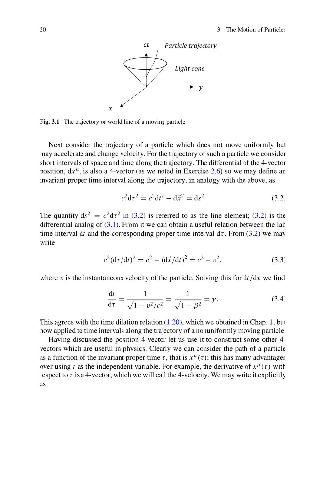
Fig. 3.1 The trajectory or world line of a moving particle
Next consider the trajectory of a particle which does not move uniformly but
may accelerate and change velocity. For the trajectory of such a particle we consider
short intervals of space and time along the trajectory. The differential of the 4-vector
position, dx
μ , is also a 4-vector (as we noted in Exercise 2.6) so we may define an
invariant proper time interval along the trajectory, in analogy with the above, as
c
2 dτ
2
= c
2 dt
2
− d x
2
= ds
2
(3.2)
The quantity ds
2
= c
2 dτ
2 in (3.2) is referred to as the line element; (3.2) is the
differential analog of (3.1). From it we can obtain a useful relation between the lab
time interval dt and the corresponding proper time interval dτ . From (3.2) we may
write
c
2
(dτ/dt)
2
= c
2
− (d x/dt)
2 = c
2
− v
2
,
(3.3)
where v is the instantaneous velocity of the particle. Solving this for dt/dτ we find
dt
dτ
=
1
1 − v 2 /c 2
=
1
1 − β 2
= γ.
(3.4)
This agrees with the time dilation relation (1.20), which we obtained in Chap. 1, but
now applied to time intervals along the trajectory of a nonuniformly moving particle.
Having discussed the position 4-vector let us use it to construct some other 4vectors which are useful in physics. Clearly we can consider the path of a particle
as a function of the invariant proper time τ , that is x
μ
(τ ); this has many advantages
over using t as the independent variable. For example, the derivative of x
μ
(τ ) with
respect to τ is a 4-vector, which we will call the 4-velocity. We may write it explicitly
as
3 The Motion of Particles
Fig. 3.1 The trajectory or world line of a moving particle
Next consider the trajectory of a particle which does not move uniformly but
may accelerate and change velocity. For the trajectory of such a particle we consider
short intervals of space and time along the trajectory. The differential of the 4-vector
position, dx
μ , is also a 4-vector (as we noted in Exercise 2.6) so we may define an
invariant proper time interval along the trajectory, in analogy with the above, as
c
2 dτ
2
= c
2 dt
2
− d x
2
= ds
2
(3.2)
The quantity ds
2
= c
2 dτ
2 in (3.2) is referred to as the line element; (3.2) is the
differential analog of (3.1). From it we can obtain a useful relation between the lab
time interval dt and the corresponding proper time interval dτ . From (3.2) we may
write
c
2
(dτ/dt)
2
= c
2
− (d x/dt)
2 = c
2
− v
2
,
(3.3)
where v is the instantaneous velocity of the particle. Solving this for dt/dτ we find
dt
dτ
=
1
1 − v 2 /c 2
=
1
1 − β 2
= γ.
(3.4)
This agrees with the time dilation relation (1.20), which we obtained in Chap. 1, but
now applied to time intervals along the trajectory of a nonuniformly moving particle.
Having discussed the position 4-vector let us use it to construct some other 4vectors which are useful in physics. Clearly we can consider the path of a particle
as a function of the invariant proper time τ , that is x
μ
(τ ); this has many advantages
over using t as the independent variable. For example, the derivative of x
μ
(τ ) with
respect to τ is a 4-vector, which we will call the 4-velocity. We may write it explicitly
as