

260
16 Some Properties of the LCDM Universe
are simple. It is called a conformal metric, as we have briefly noted previously. In this
section we will show how such a metric can be obtained for the simple example of a
flat de Sitter model universe. It will become clear that the same sort of manipulations
can be used for other models, though not as simply.
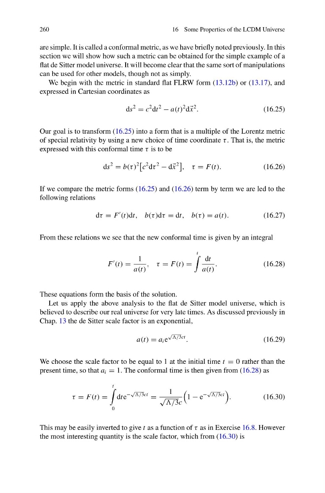
We begin with the metric in standard flat FLRW form (13.12b) or (13.17), and
expressed in Cartesian coordinates as
ds
2
= c
2 dt
2
− a(t)
2 d x
2
.
(16.25)
Our goal is to transform (16.25) into a form that is a multiple of the Lorentz metric
of special relativity by using a new choice of time coordinate τ . That is, the metric
expressed with this conformal time τ is to be
ds
2
= b(τ )
2
c
2 dτ
2
− d x
2
, τ = F(t).
(16.26)
If we compare the metric forms (16.25) and (16.26) term by term we are led to the
following relations
dτ = F
(t)dt, b(τ )dτ = dt, b(τ ) = a(t).
(16.27)
From these relations we see that the new conformal time is given by an integral
F
(t) =
1
a(t)
, τ = F(t) =
t
dt
a(t)
.
(16.28)
These equations form the basis of the solution.
Let us apply the above analysis to the flat de Sitter model universe, which is
believed to describe our real universe for very late times. As discussed previously in
Chap. 13 the de Sitter scale factor is an exponential,
a(t) = a i e
√
/3ct
.
(16.29)
We choose the scale factor to be equal to 1 at the initial time t = 0 rather than the
present time, so that a i = 1. The conformal time is then given from (16.28) as
τ = F(t) =
t
0
dte
−
√ /3ct
=
1
√
/3c
1 − e
−
√ /3ct
.
(16.30)
This may be easily inverted to give t as a function of τ as in Exercise 16.8. However
the most interesting quantity is the scale factor, which from (16.30) is
16 Some Properties of the LCDM Universe
are simple. It is called a conformal metric, as we have briefly noted previously. In this
section we will show how such a metric can be obtained for the simple example of a
flat de Sitter model universe. It will become clear that the same sort of manipulations
can be used for other models, though not as simply.
We begin with the metric in standard flat FLRW form (13.12b) or (13.17), and
expressed in Cartesian coordinates as
ds
2
= c
2 dt
2
− a(t)
2 d x
2
.
(16.25)
Our goal is to transform (16.25) into a form that is a multiple of the Lorentz metric
of special relativity by using a new choice of time coordinate τ . That is, the metric
expressed with this conformal time τ is to be
ds
2
= b(τ )
2
c
2 dτ
2
− d x
2
, τ = F(t).
(16.26)
If we compare the metric forms (16.25) and (16.26) term by term we are led to the
following relations
dτ = F
(t)dt, b(τ )dτ = dt, b(τ ) = a(t).
(16.27)
From these relations we see that the new conformal time is given by an integral
F
(t) =
1
a(t)
, τ = F(t) =
t
dt
a(t)
.
(16.28)
These equations form the basis of the solution.
Let us apply the above analysis to the flat de Sitter model universe, which is
believed to describe our real universe for very late times. As discussed previously in
Chap. 13 the de Sitter scale factor is an exponential,
a(t) = a i e
√
/3ct
.
(16.29)
We choose the scale factor to be equal to 1 at the initial time t = 0 rather than the
present time, so that a i = 1. The conformal time is then given from (16.28) as
τ = F(t) =
t
0
dte
−
√ /3ct
=
1
√
/3c
1 − e
−
√ /3ct
.
(16.30)
This may be easily inverted to give t as a function of τ as in Exercise 16.8. However
the most interesting quantity is the scale factor, which from (16.30) is